term filter 搜索数据

要搜索数据，必须得先有数据，所以接下来会先把模拟数据创建出来

创建帖子数据

根据用户ID、是否隐藏、帖子ID、发帖日期来搜索帖子

插入一些测试帖子数据

POST /forum/article/_bulk
{ "index": { "_id": 1 }}
{ "articleID" : "XHDK-A-1293-#fJ3", "userID" : 1, "hidden": false, "postDate": "2017-01-01" }
{ "index": { "_id": 2 }}
{ "articleID" : "KDKE-B-9947-#kL5", "userID" : 1, "hidden": false, "postDate": "2017-01-02" }
{ "index": { "_id": 3 }}
{ "articleID" : "JODL-X-1937-#pV7", "userID" : 2, "hidden": false, "postDate": "2017-01-01" }
{ "index": { "_id": 4 }}
{ "articleID" : "QQPX-R-3956-#aD8", "userID" : 2, "hidden": true, "postDate": "2017-01-02" }

初步来说，就先搞4个字段，因为整个 es 是支持 json document 格式的，所以说扩展性和灵活性非常之好。如果后续随着业务需求的增加，要在 document 中增加更多的 field，那么我们可以很方便的随时添加field。

但是如果是在关系型数据库中，比如mysql，我们建立了一个表，现在要给表中新增一些 column，那就很坑爹了，必须用复杂的修改表结构的语法去执行。而且可能对系统代码还有一定的影响。

查看 mappings

GET /forum/_mapping/article

响应

{
  "forum": {
    "mappings": {
      "article": {
        "properties": {
          "articleID": {
            "type": "text",
            "fields": {
              "keyword": {
                "type": "keyword",
                "ignore_above": 256
              }
            }
          },
          "hidden": {
            "type": "boolean"
          },
          "postDate": {
            "type": "date"
          },
          "userID": {
            "type": "long"
          }
        }
      }
    }
  }
}

articleID.keyword 解释

在 5.2 版本起，type = text，默认会设置两个 field：

原本的字段：articleID
不分词的字段：keyword

ignore_above：最多保留 256 个字符

可以通过 _analyze 来检测

GET /forum/_analyze
{
  "field": "articleID.keyword",
  "text": "XHDK-A-1293-#fJ3"
}

响应

{
  "error": {
    "root_cause": [
      {
        "type": "remote_transport_exception",
        "reason": "[sEvAlYx][127.0.0.1:9300][indices:admin/analyze[s]]"
      }
    ],
    "type": "illegal_argument_exception",
    "reason": "Can't process field [articleID.keyword], Analysis requests are only supported on tokenized fields"
  },
  "status": 400
}

使用 term 搜索

term：对搜索文本不分词，直接拿去倒排索引中匹配，你输入的是什么，就去匹配什么

这里就是把数据过滤出来，也不需要相关分数，可以使用 constant_score

根据用户ID搜索帖子

GET /forum/article/_search
{
  "query": {
    "constant_score": {
      "filter": {
        "term": {
          "userID": 1
        }
      }
    }
  }
}

搜索没有隐藏的帖子

GET /forum/article/_search
{
  "query": {
    "constant_score": {
      "filter": {
        "term": {
          "hidden": false
        }
      }
    }
  }
}

根据发帖日期搜索帖子

GET /forum/article/_search
{
  "query": {
    "constant_score": {
      "filter": {
        "term": {
          "postDate": "2017-01-01"
        }
      }
    }
  }
}

根据帖子ID搜索帖子

GET /forum/article/_search
{
  "query": {
    "constant_score": {
      "filter": {
        "term": {
          "articleID": "JODL-X-1937-#pV7"
        }
      }
    }
  }
}

会发现什么都搜不到

{
  "took": 2,
  "timed_out": false,
  "_shards": {
    "total": 5,
    "successful": 5,
    "failed": 0
  },
  "hits": {
    "total": 0,
    "max_score": null,
    "hits": []
  }
}

这是因为，该字段是分词字段。查看分词

查看分词

GET /forum/_analyze
{
  "field": "articleID",
  "text": "XHDK-A-1293-#fJ3"
}

响应

{
  "tokens": [
    {
      "token": "xhdk",
      "start_offset": 0,
      "end_offset": 4,
      "type": "<ALPHANUM>",
      "position": 0
    },
    {
      "token": "a",
      "start_offset": 5,
      "end_offset": 6,
      "type": "<ALPHANUM>",
      "position": 1
    },
    {
      "token": "1293",
      "start_offset": 7,
      "end_offset": 11,
      "type": "<NUM>",
      "position": 2
    },
    {
      "token": "fj3",
      "start_offset": 13,
      "end_offset": 16,
      "type": "<ALPHANUM>",
      "position": 3
    }
  ]
}

可以看到在 articleID 存储中，已经是分词的了。所以我们使用 term 不分词的肯定是匹配不上的。

前面说了 text 字段会自动 mapping 一个 keyword 字段

articleID.keyword，是 es 最新版本内置建立的 field，就是不分词的。

所以一个 articleID 过来的时候，会建立两次索引，一次是自己本身，是要分词的，分词后放入倒排索引；另外一次是基于 articleID.keyword，不分词，保留 256个字符最多，直接一个字符串放入倒排索引中。

对于 text 类型的字段就可以考虑使用 filed.keyword 字段来搜索

GET /forum/article/_search
{
  "query": {
    "constant_score": {
      "filter": {
        "term": {
          "articleID.keyword": "JODL-X-1937-#pV7"
        }
      }
    }
  }
}

结果是出来了，但是还有个问题，默认就保留 256个字符。所以尽可能还是自己去手动建立索引，指定 not_analyzed 吧。在最新版本的es中，不需要指定 not_analyzed 也可以，将 type=keyword 即可。

索引重建

DELETE /forum

PUT /forum
{
  "mappings": {
    "article":{
      "properties": {
        "articleID":{
          "type": "string",
          "index": "not_analyzed"
        }
      }
    }
  }
}

::: tip 注意 type ，如果是 text，就算指定了 index=not_analyzed 也还是会分词的。 :::

如上面这样指定之后，再次查看 mapping ，会发现被优化成了 keyword

GET /forum/_mapping

响应

{
  "forum": {
    "mappings": {
      "article": {
        "properties": {
          "articleID": {
            "type": "keyword"
          },
          "hidden": {
            "type": "boolean"
          },
          "postDate": {
            "type": "date"
          },
          "userID": {
            "type": "long"
          }
        }
      }
    }
  }
}

所以在创建索引的时候就可以直接使用 keyword 类型

PUT /forum
{
  "mappings": {
    "article":{
      "properties": {
        "articleID":{
          "type": "keyword"
        }
      }
    }
  }
}

插入测试数据之后再次搜索就可以了

知识总结

term filter：根据 exact value 进行搜索，数字、boolean、date 天然支持
text 需要建索引时指定为 not_analyzed，才能用 term query

相当于 SQL 中的单个 where 条件

  select *
  from forum.article
  where articleID='XHDK-A-1293-#fJ3'

filter 原理剖析

核心是 bitset，还有 caching 机制

1. 搜索数据，获取 document list

在倒排索引中查找搜索串，获取 document list

date 来举例

word	doc1	doc2	doc3
2017-01-01	*	*
2017-02-02		*	*
2017-03-03	*	*	*

filter：2017-02-02

到倒排索引中一找，发现 2017-02-02 对应的 document list 是 doc2,doc3

2. 构建 bitset

为每个在倒排索引中搜索到的结果，构建一个 bitset，[0, 0, 0, 1, 0, 1]

使用找到的 doc list 构建一个 bitset：就是一个二进制的数组，数组每个元素都是 0 或 1，用来标识一个 doc对一个 filter 条件是否匹配，如果匹配就是 1，不匹配就是 0

如 filter：2017-02-02 ：[0, 1, 1]

doc1：不匹配这个 filter 的
doc2 和 do3：是匹配这个 filter 的

尽可能用简单的数据结构去实现复杂的功能，可以节省内存空间，提升性能

3. 遍历 bitset，查找满足条件的 documt

遍历每个过滤条件对应的 bitset，优先从最稀疏的开始搜索，查找满足所有条件的 document

后面会讲解，一次性其实可以在一个 search 请求中，发出多个 filter 条件，每个 filter 条件都会对应一个 bitset 遍历每个 filter 条件对应的 bitset，先从最稀疏的开始遍历

[0, 0, 0, 1, 0, 0]：比较稀疏，可以简单任务是 1 最少的
[0, 1, 0, 1, 0, 1]

先遍历比较稀疏的 bitset，就可以先过滤掉尽可能多的数据；遍历所有的 bitset，找到匹配所有 filter 条件的doc

比如请求：filter，postDate=2017-01-01，userID=1

postDate: [0, 0, 1, 1, 0, 0]
userID:   [0, 1, 0, 1, 0, 1]

遍历完两个 bitset 之后，找到的匹配所有条件的 doc，就是 doc4 (都是 1)

就可以将document作为结果返回给client了

4. caching bitset

caching bitset：跟踪 query，在最近 256个 query 中超过一定次数的过滤条件，缓存其 bitset。对于小 segment（<1000，或<3%），不缓存 bitset。

比如 postDate=2017-01-01，[0, 0, 1, 1, 0, 0]，可以缓存在内存中，这样下次如果再有这个条件过来的时候，就不用重新扫描倒排索引，反复生成 bitset，可以大幅度提升性能。

在最近的 256 个 filter 中，有某个 filter 超过了一定的次数，次数不固定，就会自动缓存这个 filter 对应的 bitset

小 segment 不缓存

filter 针对小 segment 获取到的结果，可以不缓存，segment 记录数 <1000，或者 segment 大小 < index 总大小的 3%

因为：

segment 数据量很小，此时哪怕是扫描也很快；
segment 会在后台自动合并，小 segment 很快就会跟其他小 segment 合并成大 segment，此时就缓存也没有什么意义，segment 很快就消失了

filter 与 query 相比的好处

好处就是 filter 会 caching，但是之前不知道 caching 的是什么东西，实际上并不是一个 filter 返回的完整的 doc list 数据结果。而是 filter bitset 缓存起来。下次不用扫描倒排索引了。

5. filter 大部分情况下会比 query 先执行

filter 大部分情况下来说，在 query 之前执行，先尽量过滤掉尽可能多的数据

query：是会计算 doc 对搜索条件的 relevance score，还会根据这个 score 去排序
filter：只是简单过滤出想要的数据，不计算 relevance score，也不排序

::: tip 之前我一直以为 filter 是在 query 中条件查找之后，在结果上进行单纯的过滤操作。现在看来并不是这样 :::

6. 有修改或者更新，cached bitset 自动更新

如果 document 新增或修改，那么 cached bitset 会被自动更新

postDate=2017-01-01，[0, 0, 1, 0]

document，id=5，postDate=2017-01-01，会自动更新到 postDate=2017-01-01 这个 filter 的 bitset 中，全自动，缓存会自动更新。postDate=2017-01-01的bitset，[0, 0, 1, 0, 1]
document，id=1，postDate=2016-12-30，修改为 postDate-2017-01-01，此时也会自动更新 bitset，[1, 0, 1, 0, 1]

以后只要是有相同的 filter 条件的，会直接来使用这个过滤条件对应的 cached bitset

bool 组合多个 filter 搜索

第一个例子

需求如下：

搜索发帖日期为 2017-01-01 或者帖子 ID 为 XHDK-A-1293-#fJ3 的帖子
同时要求帖子的发帖日期绝对不为 2017-01-02

用 sql 来表示大致是这样

select * from forum.article
where (post_date='2017-01-01' or article_id='XHDK-A-1293-#fJ3')
and post_date!='2017-01-02'

GET /forum/article/_search
{
  "query": {
    "constant_score": {
      "filter": {
        "bool": {
          "should":[
            {"term":{"postDate":"2017-01-01"}},
            {"term":{"articleID":"XHDK-A-1293-#fJ3"}}
          ],
          "must_not":{
            "term":{
              "postDate":"2017-01-02"
            }
          }
        }
      }
    }
  }
}

::: tip 这个语法提示在 kibana 中没有提示的！！！ :::

第二个例子

搜索帖子 ID 为 XHDK-A-1293-#fJ3
或者帖子 ID 为 JODL-X-1937-#pV7 而且发帖日期为 2017-01-01 的帖子

select * from forum.article
where article_id='XHDK-A-1293-#fJ3'
or (article_id='JODL-X-1937-#pV7' and post_date='2017-01-01')

GET /forum/article/_search
{
  "query": {
    "constant_score": {
      "filter": {
        "bool": {
          "should":[
            {"term":{"articleID":"XHDK-A-1293-#fJ3"}},
            {"bool":{
                "must":[
                  {"term":{"articleID":"JODL-X-1937-#pV7"}},
                  {"term":{"postDate":"2017-01-01"}}
                ]
              }
            }
          ]
        }
      }
    }
  }
}

总结

bool：must，must_not，should，组合多个过滤条件
bool 可以嵌套
相当于 SQL 中的多个 and 条件：当你把搜索语法学好了以后，基本可以实现部分常用的 sql 语法对应的功能

::: tip 好多语法提示在 kibana 中没有提示的！！！，重要的事情多说几遍，以前一直以为没有提示就是不支持 :::

terms 搜索多个值

之前都是使用 term 搜索一个词，那么怎么实现 sql 中的 in 效果呢？

select * from tbl where col in ("value1", "value2")

就可以使用 terms

terms: {"field": ["value1", "value2"]}

为帖子数据增加 tag 字段；增加模拟数据

POST /forum/article/_bulk
{ "update": { "_id": "1"} }
{ "doc" : {"tag" : ["java", "hadoop"]} }
{ "update": { "_id": "2"} }
{ "doc" : {"tag" : ["java"]} }
{ "update": { "_id": "3"} }
{ "doc" : {"tag" : ["hadoop"]} }
{ "update": { "_id": "4"} }
{ "doc" : {"tag" : ["java", "elasticsearch"]} }

搜索 articleID 为 KDKE-B-9947-#kL5 或 QQPX-R-3956-#aD8的帖子

GET /forum/article/_search
{
  "query": {
    "constant_score": {
      "filter": {
        "terms": {
          "articleID": [
            "KDKE-B-9947-#kL5",
            "QQPX-R-3956-#aD8"
          ]
        }
      }
    }
  }
}

搜索 tag 中包含 java 的帖子

由于这里只有一个条件，所以使用 term ，而不是 terms

GET /forum/article/_search
{
  "query": {
    "constant_score": {
      "filter": {
        "term": {
          "tag": "java"
        }
      }
    }
  }
}

响应结果

{
  "took": 1,
  "timed_out": false,
  "_shards": {
    "total": 5,
    "successful": 5,
    "failed": 0
  },
  "hits": {
    "total": 3,
    "max_score": 1,
    "hits": [
      {
        "_index": "forum",
        "_type": "article",
        "_id": "2",
        "_score": 1,
        "_source": {
          "articleID": "KDKE-B-9947-#kL5",
          "userID": 1,
          "hidden": false,
          "postDate": "2017-01-02",
          "tag": [
            "java"
          ]
        }
      },
      {
        "_index": "forum",
        "_type": "article",
        "_id": "4",
        "_score": 1,
        "_source": {
          "articleID": "QQPX-R-3956-#aD8",
          "userID": 2,
          "hidden": true,
          "postDate": "2017-01-02",
          "tag": [
            "java",
            "elasticsearch"
          ]
        }
      },
      {
        "_index": "forum",
        "_type": "article",
        "_id": "1",
        "_score": 1,
        "_source": {
          "articleID": "XHDK-A-1293-#fJ3",
          "userID": 1,
          "hidden": false,
          "postDate": "2017-01-01",
          "tag": [
            "java",
            "hadoop"
          ]
        }
      }
    ]
  }
}

可见如上结果，tag 中包含 java 的都出来了，那么如果只包含 java 的呢？

搜索 tag 只包含 java 的帖子

该需求在目前的知识中貌似实现不了呢，可以通过一个标识字段来实现。

标识当前 tag 中 tag 的数量，只要为 1 的且又包含 java 的就可以了

增加 tag 数量字段

POST /forum/article/_bulk
{ "update": { "_id": "1"} }
{ "doc" : {"tag_cnt" : 2} }
{ "update": { "_id": "2"} }
{ "doc" : {"tag_cnt" : 1} }
{ "update": { "_id": "3"} }
{ "doc" : {"tag_cnt" : 1} }
{ "update": { "_id": "4"} }
{ "doc" : {"tag_cnt" : 2} }

GET /forum/article/_search
{
  "query": {
    "constant_score": {
      "filter": {
        "bool": {
          "must":[
            {"term":{
              "tag":"java"
            }},
            {
              "match": {
                "tag_cnt": 1
              }
            }
          ]
        }
      }
    }
  }
}

查找 tag 中只包含 java 和 hadoop 的数据

GET /forum/article/_search
{
  "query": {
    "constant_score": {
      "filter": {
        "bool": {
          "must":[
            {"term":{
              "tag":"java"
            }},
            {"term":{
              "tag":"hadoop"
            }},
            {
              "match": {
                "tag_cnt": 2
              }
            }
          ]
        }
      }
    }
  }
}

使用 must + 2个 term 限制至少该数据包含 java 和 hadoop
并且他们的数量只能为 2

响应

{
  "took": 1,
  "timed_out": false,
  "_shards": {
    "total": 5,
    "successful": 5,
    "failed": 0
  },
  "hits": {
    "total": 1,
    "max_score": 1,
    "hits": [
      {
        "_index": "forum",
        "_type": "article",
        "_id": "1",
        "_score": 1,
        "_source": {
          "articleID": "XHDK-A-1293-#fJ3",
          "userID": 1,
          "hidden": false,
          "postDate": "2017-01-01",
          "tag": [
            "java",
            "hadoop"
          ],
          "tag_cnt": 2
        }
      }
    ]
  }
}

总结

terms 多值搜索
优化 terms 多值搜索的结果
相当于 SQL 中的 in 语句
range filter 范围过滤

为帖子增加浏览量的字段数据

POST /forum/article/_bulk
{ "update": { "_id": "1"} }
{ "doc" : {"view_cnt" : 30} }
{ "update": { "_id": "2"} }
{ "doc" : {"view_cnt" : 50} }
{ "update": { "_id": "3"} }
{ "doc" : {"view_cnt" : 100} }
{ "update": { "_id": "4"} }
{ "doc" : {"view_cnt" : 80} }

数值范围查询

搜索浏览量在 30~60 之间的帖子

GET /forum/article/_search
{
  "query": {
    "constant_score": {
      "filter": {
        "range": {
          "view_cnt": {
            "gte": 30,
            "lte": 60
          }
        }
      }
    }
  }
}

gt：大于
lt：小于
gte：大于等于
lte：小于等于

日期范围查询

搜索发帖日期在最近 1个月的帖子

由于该笔记是 2019.01.28 记录的，需要添加一条记录

POST /forum/article/_bulk
{ "index": { "_id": 5 }}
{ "articleID" : "DHJK-B-1395-#Ky5", "userID" : 3, "hidden": false, "postDate": "2019-01-28", "tag": ["elasticsearch"], "tag_cnt": 1, "view_cnt": 10 }

最近一个月：也就是当前时间 - 30天，大于该时间即可

GET /forum/article/_search
{
  "query": {
    "constant_score": {
      "filter": {
        "range": {
          "postDate": {
            "gte": "2018-01-01"
          }
        }
      }
    }
  }
}

上面这个时间是我们自己算的，es 支持动态语法

now-30d：当前时间减去 30天
2019-01-30 -2d：下面例子来说 gte：

大于 2019.01.30 或者是大于 2019.01.30 -2 天 = 2019.01.28

GET /forum/article/_search
{
  "query": {
    "constant_score": {
      "filter": {
        "range": {
          "postDate": {
            "gte": "2019-01-30||-2d"
          }
        }
      }
    }
  }
}

总结

range，sql 中的 between，或者是 >=1，<=1
range 做范围过滤
体验如何控制全文检索结果的精准度

增加测试数据，添加一个 title 字段

POST /forum/article/_bulk
{ "update": { "_id": "1"} }
{ "doc" : {"title" : "this is java and elasticsearch blog"} }
{ "update": { "_id": "2"} }
{ "doc" : {"title" : "this is java blog"} }
{ "update": { "_id": "3"} }
{ "doc" : {"title" : "this is elasticsearch blog"} }
{ "update": { "_id": "4"} }
{ "doc" : {"title" : "this is java, elasticsearch, hadoop blog"} }
{ "update": { "_id": "5"} }
{ "doc" : {"title" : "this is spark blog"} }

1、搜索标题中包含 java 或 elasticsearch 的 blog

term query：搜索 exact value
match query：full text 全文检索

如果要检索的 field，是 not_analyzed 类型的，那么 match query 也相当于 term query。

GET /forum/article/_search
{
    "query": {
        "match": {
            "title": "java elasticsearch"
        }
    }
}

会出来 4 条数据。

2、搜索标题中包含 java 和 elasticsearch 的 blog

GET /forum/article/_search
{
    "query": {
        "match": {
            "title": {
          		"query": "java elasticsearch",
          		"operator": "and"
   	        }
        }
    }
}

搜索的结果是包含 java 和 elasticsearch 两个关键词的结果，并不是 term query 的精准匹配

3、搜索包含 java、elasticsearch、spark、hadoop 4 个关键字中，至少 3 个的 blog

GET /forum/article/_search
{
    "query": {
        "match": {
            "title": {
          		"query": "java elasticsearch spark hadoop",
          		"minimum_should_match": "75%"
   	        }
        }
    }
}

minimum_should_match：必须至少匹配其中的多少个关键字，才能作为结果返回，默认是一个

4、用 bool 组合多个搜索条件，来搜索 title

GET /forum/article/_search
{
  "query": {
    "bool": {
      "must":     { "match": { "title": "java" }},
      "must_not": { "match": { "title": "spark"  }},
      "should": [
          { "match": { "title": "hadoop" }},
          { "match": { "title": "elasticsearch"   }}
      ]
    }
  }
}

再来解说下这个：必须包含 java，且不能包含 spark，且可以包含或者不包含 hadoop 和 elasticsearch；

这里的 should 这样用我觉得没有什么必要，那有什么用么？下面会讲解相关作用

5、bool 组合多个搜索条件，如何计算 relevance score

must 和 should 搜索对应的分数，加起来，除以 must 和 should 的总数

排名第一：java，同时包含 should 中所有的关键字，hadoop，elasticsearch
排名第二：java，同时包含 should 中的 elasticsearch
排名第三：java，不包含 should 中的任何关键字

should 是可以影响相关度分数的

must 是确保说，谁必须有这个关键字，同时会根据这个 must 的条件去计算出 document 对这个搜索条件的 relevance score

在满足 must 的基础之上，should 中的条件，不匹配也可以，但是如果匹配的更多，那么 document 的 relevance score 就会更高

看下面的结果排名，对照上面的就清楚了

"hits": [
      {
        "_index": "forum",
        "_type": "article",
        "_id": "4",
        "_score": 1.3375794,
        "_source": {
          "articleID": "QQPX-R-3956-#aD8",
          "userID": 2,
          "hidden": true,
          "postDate": "2017-01-02",
          "tag": [
            "java",
            "elasticsearch"
          ],
          "tag_cnt": 2,
          "view_cnt": 80,
          "title": "this is java, elasticsearch, hadoop blog"
        }
      },
      {
        "_index": "forum",
        "_type": "article",
        "_id": "1",
        "_score": 0.53484553,
        "_source": {
          "articleID": "XHDK-A-1293-#fJ3",
          "userID": 1,
          "hidden": false,
          "postDate": "2017-01-01",
          "tag": [
            "java",
            "hadoop"
          ],
          "tag_cnt": 2,
          "view_cnt": 30,
          "title": "this is java and elasticsearch blog"
        }
      },
      {
        "_index": "forum",
        "_type": "article",
        "_id": "2",
        "_score": 0.19856805,
        "_source": {
          "articleID": "KDKE-B-9947-#kL5",
          "userID": 1,
          "hidden": false,
          "postDate": "2017-01-02",
          "tag": [
            "java"
          ],
          "tag_cnt": 1,
          "view_cnt": 50,
          "title": "this is java blog"
        }
      }
    ]

6、搜索 java、hadoop、spark、elasticsearch，至少包含其中 3 个关键字

至少满足 should 中的 3个条件才返回结果

GET /forum/article/_search
{
  "query": {
    "bool": {
      "should": [
        { "match": { "title": "java" }},
        { "match": { "title": "elasticsearch"   }},
        { "match": { "title": "hadoop"   }},
	      { "match": { "title": "spark"   }}
      ],
      "minimum_should_match": 3
    }
  }
}

总结

全文检索的时候，进行多个值的检索，有两种做法，
- match query
- should
控制搜索结果精准度：
- operator and
- minimum_should_match
  多关键词底层原理 term + bool

普通 match 如何转换为 term + should？

{
    "match": { "title": "java elasticsearch"}
}

使用诸如上面的 match query 进行多值搜索的时候，es 会在底层自动将这个 match query 转换为 bool 的语法 bool should，指定多个搜索词，同时使用 term query

{
  "bool": {
    "should": [
      { "term": { "title": "java" }},
      { "term": { "title": "elasticsearch"}}
    ]
  }
}

and match 如何转换为 term + must？

{
    "match": {
        "title": {
            "query":    "java elasticsearch",
            "operator": "and"
        }
    }
}
转换为
{
  "bool": {
    "must": [
      { "term": { "title": "java" }},
      { "term": { "title": "elasticsearch"   }}
    ]
  }
}

minimum_should_match 如何转换

{
    "match": {
        "title": {
            "query":                "java elasticsearch hadoop spark",
            "minimum_should_match": "75%"
        }
    }
}
转换为
{
  "bool": {
    "should": [
      { "term": { "title": "java" }},
      { "term": { "title": "elasticsearch"   }},
      { "term": { "title": "hadoop" }},
      { "term": { "title": "spark" }}
    ],
    "minimum_should_match": 3
  }
}

上一讲，为啥要讲解两种实现 multi-value 搜索的方式呢？实际上，就是给这一讲进行铺垫的。match query –> bool + term。

权重控制 boost

权重是什么意思呢？简单来说就是用数值来给「重要」量化

比如这个需求：

搜索标题中包含 java 的帖子
同时呢，如果标题中包含 hadoop 或 elasticsearch 就优先搜索出来，
同时呢，如果一个帖子包含 java hadoop，一个帖子包含 java elasticsearch，包含 hadoop 的帖子要比 elasticsearch 优先搜索出来

知识点：boost 搜索条件的权重，可以将某个搜索条件的权重加大，此时当匹配这个搜索条件和匹配另一个搜索条件的 document，计算 relevance score 时，匹配权重更大的搜索条件的 document，relevance score 会更高，当然也就会优先被返回回来

默认情况下，搜索条件的权重都是一样的，都是 1

比如下面这个查询，前面讲到过 should 的的得分计算，如果 spark 的 boost=1 那么 “title”: “this is java, elasticsearch, hadoop blog” 肯定是得分最高的，因为满足个数最多。

下面这个查询结果由于 spark 的 boost=5，最高得分就是 “title”: “this is spark blog” 了，

::: tip 得分有相关的计算，权重只是提高了这个分支，可以理解为最终得分再多加这个权重分，而不是直接手动排序 :::

GET /forum/article/_search
{
  "query": {
    "bool": {
      "must": [
        {
          "match": {
            "title": "blog"
          }
        }
      ],
      "should": [
        {
          "match": {
            "title": {
              "query": "java"
            }
          }
        },
        {
          "match": {
            "title": {
              "query": "hadoop"
            }
          }
        },
        {
          "match": {
            "title": {
              "query": "elasticsearch"
            }
          }
        },
        {
          "match": {
            "title": {
              "query": "spark",
              "boost": 5
            }
          }
        }
      ]
    }
  }
}

多 shard 下评分不准确大揭秘

得分不准的产生

1 个 index 有多个 shard（副本）的情况下，有时会导致 relevance score 不准确的情况；

那么这个情况是怎么产生的呢？es 官网自己说该得分计算是有一点问题的（不知道哪里写的），

在相关度评分 TF&IDF 算法独家解密中有讲到过得分的计算规则。# dis_max 实现 best fields 策略多字段搜索

增加 content 字段的测试数据

POST /forum/article/_bulk
{ "update": { "_id": "1"} }
{ "doc" : {"content" : "i like to write best elasticsearch article"} }
{ "update": { "_id": "2"} }
{ "doc" : {"content" : "i think java is the best programming language"} }
{ "update": { "_id": "3"} }
{ "doc" : {"content" : "i am only an elasticsearch beginner"} }
{ "update": { "_id": "4"} }
{ "doc" : {"content" : "elasticsearch and hadoop are all very good solution, i am a beginner"} }
{ "update": { "_id": "5"} }
{ "doc" : {"content" : "spark is best big data solution based on scala ,an programming language similar to java"} }

问题产生

搜索 title 或 content 中包含 java 或 solution 的帖子

GET /forum/article/_search
{
  "query": {
    "bool": {
      "should": [
        {"match": {
          "title": "java solution"
        }},
        {
          "match": {
            "content": "java solution"
          }
        }
      ]
    }
  }
}

获取其中两条数据来分析下为什么会这样？下面两条数据比较好描述

id 5 的 doc 中 content 包含了 solution 和 java，而 id 4 中只包含一个词语，应该是 id 5 得分高才对吧？

id=4，得分 0.7120095
"title": "this is java, elasticsearch, hadoop blog",
"content": "elasticsearch and hadoop are all very good solution, i am a beginner"

id=5，得分 0.56008905
"title": "this is spark blog",
"content": "spark is best big data solution based on scala ,an programming language similar to java"

这个就关系到 es 中的 should 得分计算规则有关系了。大体的公式可以理解为这样：每个 query 得分相加 * matched query 数量 / 总 query 数量。

如 id 4 ：

- title 中包含 java ； matched query 有得分，假设是 1.1
- content 中包含 solution；matched query 有得分，假设是 1.2
- matched query 数量：就是有得分的 query 数量，这里为 2
- 总 query 数量：should 中的 query 个数，这里为 2

(1.1 + 1.2) * 2 / 2 = 2.3

id 4：

- title ：没有得分
- content 中包含 solution 和 java 有得分，假设是 2.3
- matched query 数量：就是有得分的 query 数量，这里为 1
- 总 query 数量：should 中的 query 个数，这里为 2

2.3 * 1 / 2 = 1.5

这里就看出来了，id 5 得分变低了

best fields 策略和 dis_max

best fields 策略：某一个 field 中匹配到了尽可能多的关键词，得分就高
dis_max 语法：直接取多个 query 中，分数最高的那一个 query 的分数即可

有这两项保证，就能得到我们想要的结果了

GET /forum/article/_search
{
  "query": {
    "dis_max": {
      "queries": [
          {"match": {
          "title": "java solution"
        }},
        {
          "match": {
            "content": "java solution"
          }
        }
      ]
    }
  }
}

dis_max 的 tie_breaker 作用

GET /forum/article/_search
{
    "query": {
        "dis_max": {
            "queries": [
                { "match": { "title": "java beginner" }},
                { "match": { "body":  "java beginner" }}
            ],
            "tie_breaker": 0.3
        }
    }
}

用法如上，那么 tie_breaker 有什么作用呢？

如果你仔细观察使用 tie_breaker 和不使用查询出来的某一条数据的 _score 分数就能看出来了，添加了之后会相应的提高。

dis_max 就是获取得分最高的那一个 query，这样就一刀切了，在某些情况下就会导致结果不是正确的；

title 中包含 java ； matched query 有得分，假设是 1.1
content 中包含 solution；matched query 有得分，假设是 1.2

添加了 tie_breaker = 0.3，那么就是这样的了， 1.1 * 0.3 + 1.2 = 1.53；

大于 dis_max 获取最高一条得分的 1.2，这样一来关联性就会上去了，也就会更合理一点

multi_match 语法

例如这样一个查询，使用 dis_max 语法的

GET /forum/article/_search
{
  "query": {
    "dis_max": {
      "queries":  [
        {
          "match": {
            "title": {
              "query": "java beginner",
              "minimum_should_match": "50%",
	            "boost": 2
            }
          }
        },
        {
          "match": {
            "content": {
              "query": "java beginner",
              "minimum_should_match": "30%"
            }
          }
        }
      ],
      "tie_breaker": 0.3
    }
  }
}

dis_max：获取得分最高的一个 query 作为最终得分
tie_breaker：综合其他 query 得分，也可以理解为一点权重的意思吧
boost：权重
minimum_should_match：去长尾

什么意思呢？举个例子，查询「java is good bee」，但是某些结果可能只包含了一个 java 这样一来关联性就很低了，设置必须满足一定的个数才算匹配该条件，这个就是去长尾

上面这个可以使用 multi_match 语法来转化

GET /forum/article/_search
{
  "query": {
    "multi_match": {
        "query":                "java beginner",
        "type":                 "best_fields",
        "fields":               [ "title^2", "content" ],
        "tie_breaker":          0.3,
        "minimum_should_match": "50%"
    }
  }
}

title^2：来表示 boots
multi_match 的 most_fiels 策略
most-fiels: 在多个 field 查询到关键词的则优先返回该 doc
best_fields：在一个 field 中匹配到多个查询词的则优先返回该 doc

他们两个是刚好相反的一个策略

现在来实验，首先添加测试数据

POST /forum/article/_bulk
{ "update": { "_id": "1"} }
{ "doc" : {"sub_title" : "learning more courses"} }
{ "update": { "_id": "2"} }
{ "doc" : {"sub_title" : "learned a lot of course"} }
{ "update": { "_id": "3"} }
{ "doc" : {"sub_title" : "we have a lot of fun"} }
{ "update": { "_id": "4"} }
{ "doc" : {"sub_title" : "both of them are good"} }
{ "update": { "_id": "5"} }
{ "doc" : {"sub_title" : "haha, hello world"} }

GET /forum/article/_search
{
  "query": {
    "match": {
      "sub_title": "learning courses"
    }
  }
}

这个查询出来的结果我们希望是 id=1 的数据会排在最前面，因为最相关。但是使用默认的 mapping 就不一定

原理就是：sub_title 会自动 mapping 成 enligsh analyzer，所以还原了单词

为什么，因为如果我们用的是类似于 english analyzer 这种分词器的话，就会将单词还原为其最基本的形态（stemmer）

learning --> learn
learned --> learn
courses --> course

sub_titile: learning coureses --> learn course

这样转换后再查询，相关分就和我们想象的不太一样了。所以先处理该差异，手动 mapping

POST /forum/_mapping/article
{
  "properties": {
      "sub_title": {
          "type":     "string",
          "analyzer": "english",
          "fields": {
              "std":   {
                  "type":     "string",
                  "analyzer": "standard"
              }
          }
      }
  }
}

再次查询

GET /forum/article/_search
{
  "query": {
    "match": {
      "sub_title.std": "learning courses"
    }
  }
}

就只会返回一条了，因为只有这一条符合标准

{
  "took": 2,
  "timed_out": false,
  "_shards": {
    "total": 5,
    "successful": 5,
    "failed": 0
  },
  "hits": {
    "total": 1,
    "max_score": 0.5063205,
    "hits": [
      {
        "_index": "forum",
        "_type": "article",
        "_id": "1",
        "_score": 0.5063205,
        "_source": {
          "articleID": "XHDK-A-1293-#fJ3",
          "userID": 1,
          "hidden": false,
          "postDate": "2017-01-01",
          "tag": [
            "java",
            "hadoop"
          ],
          "tag_cnt": 2,
          "view_cnt": 30,
          "title": "this is java and elasticsearch blog",
          "content": "i like to write best elasticsearch article",
          "sub_title": "learning more courses"
        }
      }
    ]
  }
}

如果不使用 .std 就会使用分词形式去匹配到两条数据。multi_match 语法如下

GET /forum/article/_search
{
   "query": {
        "multi_match": {
            "query":  "learning courses",
            "type":   "most_fields",
            "fields": [ "sub_title", "sub_title.std" ]
        }
    }
}

响应结果

{
  "took": 3,
  "timed_out": false,
  "_shards": {
    "total": 5,
    "successful": 5,
    "failed": 0
  },
  "hits": {
    "total": 2,
    "max_score": 1.219939,
    "hits": [
      {
        "_index": "forum",
        "_type": "article",
        "_id": "2",
        "_score": 1.219939,
        "_source": {
          "articleID": "KDKE-B-9947-#kL5",
          "userID": 1,
          "hidden": false,
          "postDate": "2017-01-02",
          "tag": [
            "java"
          ],
          "tag_cnt": 1,
          "view_cnt": 50,
          "title": "this is java blog",
          "content": "i think java is the best programming language",
          "sub_title": "learned a lot of course"
        }
      },
      {
        "_index": "forum",
        "_type": "article",
        "_id": "1",
        "_score": 1.012641,
        "_source": {
          "articleID": "XHDK-A-1293-#fJ3",
          "userID": 1,
          "hidden": false,
          "postDate": "2017-01-01",
          "tag": [
            "java",
            "hadoop"
          ],
          "tag_cnt": 2,
          "view_cnt": 30,
          "title": "this is java and elasticsearch blog",
          "content": "i like to write best elasticsearch article",
          "sub_title": "learning more courses"
        }
      }
    ]
  }
}

但是这还是没有出现我们希望的结果是为什么呢？这个老师也讲解不清楚了，计算很复杂；但是有一点可以知道，使用 best_fields 和 most_fields 查看对于 id=1 的评分，在 most_fields 策略下评分达到了 1+ ，而 best_fields 策略下只有 0.5+；

这就可以说明 most_fields 策略的作用了

GET /forum/article/_search
{
   "query": {
        "multi_match": {
            "query":  "learning courses",
            "type":   "best_fields",
            "fields": [ "sub_title", "sub_title.std" ]
        }
    }
}

most_fields 策略 cross-fields 搜索弊端

cross-fields （跨字段）搜索：一个唯一标识，跨了多个 field。比如一个人，标识，是姓名；一个建筑，它的标识是地址。姓名可以散落在多个 field 中，比如 first_name 和 last_name 中，地址可以散落在 country、province、city中。

跨多个 field 搜索一个标识，比如搜索一个人名，或者一个地址，就是 cross-fields 搜索

初步来说，如果要实现，可能用 most_fields 比较合适。因为 best_fields 是优先搜索单个 field 最匹配的结果， cross-fields 本身就不是一个 field 的问题了。

增加字段数据

POST /forum/article/_bulk
{ "update": { "_id": "1"} }
{ "doc" : {"author_first_name" : "Peter", "author_last_name" : "Smith"} }
{ "update": { "_id": "2"} }
{ "doc" : {"author_first_name" : "Smith", "author_last_name" : "Williams"} }
{ "update": { "_id": "3"} }
{ "doc" : {"author_first_name" : "Jack", "author_last_name" : "Ma"} }
{ "update": { "_id": "4"} }
{ "doc" : {"author_first_name" : "Robbin", "author_last_name" : "Li"} }
{ "update": { "_id": "5"} }
{ "doc" : {"author_first_name" : "Tonny", "author_last_name" : "Peter Smith"} }

查询

GET /forum/article/_search
{
  "query": {
    "multi_match": {
      "query":       "Peter Smith",
      "type":        "most_fields",
      "fields":      [ "author_first_name", "author_last_name" ]
    }
  }
}

响应结果

{
  "took": 118,
  "timed_out": false,
  "_shards": {
    "total": 5,
    "successful": 5,
    "failed": 0
  },
  "hits": {
    "total": 3,
    "max_score": 0.6931472,
    "hits": [
      {
        "_index": "forum",
        "_type": "article",
        "_id": "2",
        "_score": 0.6931472,
        "_source": {
          "articleID": "KDKE-B-9947-#kL5",
          "userID": 1,
          "hidden": false,
          "postDate": "2017-01-02",
          "tag": [
            "java"
          ],
          "tag_cnt": 1,
          "view_cnt": 50,
          "title": "this is java blog",
          "content": "i think java is the best programming language",
          "sub_title": "learned a lot of course",
          "author_first_name": "Smith",
          "author_last_name": "Williams"
        }
      },
      {
        "_index": "forum",
        "_type": "article",
        "_id": "1",
        "_score": 0.5753642,
        "_source": {
          "articleID": "XHDK-A-1293-#fJ3",
          "userID": 1,
          "hidden": false,
          "postDate": "2017-01-01",
          "tag": [
            "java",
            "hadoop"
          ],
          "tag_cnt": 2,
          "view_cnt": 30,
          "title": "this is java and elasticsearch blog",
          "content": "i like to write best elasticsearch article",
          "sub_title": "learning more courses",
          "author_first_name": "Peter",
          "author_last_name": "Smith"
        }
      },
      {
        "_index": "forum",
        "_type": "article",
        "_id": "5",
        "_score": 0.51623213,
        "_source": {
          "articleID": "DHJK-B-1395-#Ky5",
          "userID": 3,
          "hidden": false,
          "postDate": "2019-01-28",
          "tag": [
            "elasticsearch"
          ],
          "tag_cnt": 1,
          "view_cnt": 10,
          "title": "this is spark blog",
          "content": "spark is best big data solution based on scala ,an programming language similar to java",
          "sub_title": "haha, hello world",
          "author_first_name": "Tonny",
          "author_last_name": "Peter Smith"
        }
      }
    ]
  }
}

会发现 id=5 的 "author_last_name": "Peter Smith" 居然是排在最后面的，我们想要的结果应该就是 id=5 这条数据了，造成这个结果的原因如下：

只是找到尽可能多的 field 匹配的 doc，而不是某个 field 完全匹配的 doc
most_fields 没办法用 minimum_should_match 去掉长尾数据，就是匹配的特别少的结果
TF/IDF算法，

比如 Peter Smith 和 Smith Williams，搜索 Peter Smith 的时候，由于 first_name 中很少有 Smith 的，所以 query 在所有 document 中的频率很低，得到的分数很高，可能 Smith Williams 反而会排在 Peter Smith 前面

注意：该算法在本教程中有时候的解释并不是完全正确，只大概是这样

copy_to 解决 cross-fields

上一节使用 most_fields 来解决多字段搜索的需求的弊端中最最核心的问题就是有跨字段搜索了，那么这里就可以使用 copy_to 来让多个字段组合成一个字段

需要先 mapping ，这里新增加字段

PUT /forum/_mapping/article
{
  "properties": {
      "new_author_first_name": {
          "type":     "string",
          "copy_to":  "new_author_full_name"
      },
      "new_author_last_name": {
          "type":     "string",
          "copy_to":  "new_author_full_name"
      },
      "new_author_full_name": {
          "type":     "string"
      }
  }
}

再增加数据

POST /forum/article/_bulk
{ "update": { "_id": "1"} }
{ "doc" : {"new_author_first_name" : "Peter", "new_author_last_name" : "Smith"} }		
{ "update": { "_id": "2"} }
{ "doc" : {"new_author_first_name" : "Smith", "new_author_last_name" : "Williams"} }		
{ "update": { "_id": "3"} }
{ "doc" : {"new_author_first_name" : "Jack", "new_author_last_name" : "Ma"} }		
{ "update": { "_id": "4"} }
{ "doc" : {"new_author_first_name" : "Robbin", "new_author_last_name" : "Li"} }		
{ "update": { "_id": "5"} }
{ "doc" : {"new_author_first_name" : "Tonny", "new_author_last_name" : "Peter Smith"} }	 

注意：在查询的时候 new_author_full_name 字段并不会显示出来，在查询 mapping 的时候才能看到

::: warning 该章节示例的测试不能解决我们的需求，因为该打分的的策略没有彻底搞明白的缘故。所以复现不出来了 :::

这几章节的内容其实就是讲解了什么场景下使用：best_fields、most_fields

cross-fields

在 multi_match 中就已经支持了 cross_fields

GET /forum/article/_search
{
  "query": {
    "multi_match": {
      "query": "Peter Smith",
      "type": "cross_fields",
      "operator": "and",
      "fields": ["author_first_name", "author_last_name"]
    }
  }
}

响应结果

{
  "took": 7,
  "timed_out": false,
  "_shards": {
    "total": 5,
    "successful": 5,
    "failed": 0
  },
  "hits": {
    "total": 2,
    "max_score": 0.5753642,
    "hits": [
      {
        "_index": "forum",
        "_type": "article",
        "_id": "1",
        "_score": 0.5753642,
        "_source": {
          "articleID": "XHDK-A-1293-#fJ3",
          "userID": 1,
          "hidden": false,
          "postDate": "2017-01-01",
          "tag": [
            "java",
            "hadoop"
          ],
          "tag_cnt": 2,
          "view_cnt": 30,
          "title": "this is java and elasticsearch blog",
          "content": "i like to write best elasticsearch article",
          "sub_title": "learning more courses",
          "author_first_name": "Peter",
          "author_last_name": "Smith",
          "new_author_last_name": "Smith",
          "new_author_first_name": "Peter"
        }
      },
      {
        "_index": "forum",
        "_type": "article",
        "_id": "5",
        "_score": 0.51623213,
        "_source": {
          "articleID": "DHJK-B-1395-#Ky5",
          "userID": 3,
          "hidden": false,
          "postDate": "2019-01-28",
          "tag": [
            "elasticsearch"
          ],
          "tag_cnt": 1,
          "view_cnt": 10,
          "title": "this is spark blog",
          "content": "spark is best big data solution based on scala ,an programming language similar to java",
          "sub_title": "haha, hello world",
          "author_first_name": "Tonny",
          "author_last_name": "Peter Smith",
          "new_author_last_name": "Peter Smith",
          "new_author_first_name": "Tonny"
        }
      }
    ]
  }
}

和最开始说想要 id=5 的数据还是没能达到要求，但是现在的结果已经很正常了。无论是单独还是组合都出现了 Peter Smith，其他的还是评分缘故

match_phrase 短语匹配

什么是短语匹配和近似匹配？

先来看一个搜索例子

添加两条数据

PUT /forum/article/6
{
  "content":"java is my favourite programming language, and I also think spark is a very good big data system."
}

PUT /forum/article/7
{
  "content":"java spark are very related, because scala is spark's programming language and scala is also based on jvm like java."
}

PUT /forum/article/8
{
  "content":"java are spark very related, because scala is spark's programming language and scala is also based on jvm like java."
}

查询

GET /forum/article/_search
{
  "query": {
      "match": {
        "content": "java spark"
      }
    }
  }
}

会看到这三条数据都返回来了，并且 id=7 的得分要高于 id=6 的。

假如要实现下面需求：

java spark，就靠在一起，中间不能插入任何其他字符，就要搜索出来这种 doc
java spark，但是要求，java 和 spark 两个单词靠的越近，doc 的分数越高，排名越靠前

使用 match 是搞不定的，match 只能搜索到包含 java 和 spark 的数据（因为会分词成两个词）

近似匹配包括以下两类，短语匹配也属于近似匹配，后续会看到（如 slop）

phrase match 短语匹配：就是不分词，直接包含这个词的
proximity match 近似匹配：靠得越近得分越高

phrase match

GET /forum/article/_search
{
  "query": {
      "match_phrase": {
        "content": "java spark"
      }
    }
  }
}

成功了，只有包含 java spark 这个短语的 doc 才返回了，只包含 java 的 doc 不会返回

term position

什么是 term position？简单说就是分词后的词在原始 doc 中的顺序位置

通过下面的的语法可以查看到分词后的 position

GET _analyze
{
  "text": "hello world, java spark",
  "analyzer": "standard"
}

GET _analyze
{
  "text": "hi, spark java",
  "analyzer": "standard"
}

其中一个返回

{
  "tokens": [
    {
      "token": "hello",
      "start_offset": 0,
      "end_offset": 5,
      "type": "<ALPHANUM>",
      "position": 0
    },
    {
      "token": "world",
      "start_offset": 6,
      "end_offset": 11,
      "type": "<ALPHANUM>",
      "position": 1
    },
    {
      "token": "java",
      "start_offset": 13,
      "end_offset": 17,
      "type": "<ALPHANUM>",
      "position": 2
    },
    {
      "token": "spark",
      "start_offset": 18,
      "end_offset": 23,
      "type": "<ALPHANUM>",
      "position": 3
    }
  ]
}

phrase match 基本原理

倒排索引中的 position 示例

hello world, java spark		doc1
hi, spark java				 doc2

--- 倒排索引示例，
hello   doc1(0)		
wolrd   doc1(1)
java    doc1(2) doc2(2)
spark   doc1(3) doc2(1)

java spark --> java 和 spark
match phrase 要求 doc 必须包含所有的关键词才符合第一步条件

--- 查询词在 doc 中的 position 示例
java -->  doc1(2) doc2(2)
spark --> doc1(3) doc2(1)

对于 match phrase 来说，spark 的 position > java 的 position 且必须大于 1 才能满足条件。因为刚好大于 1 的话，就能拼接成 java spark。

通过 position 的对比就能判定这个搜索是否是一个短语

这样看来，后面的 proximity match 原理也应该是这样！

match_phrase 的 slop

语法

GET /forum/article/_search
{
    "query": {
        "match_phrase": {
            "content": {
                "query": "java spark",
                "slop":  1
            }
        }
    }
}

slop 的含义是什么？

query string 搜索文本中的几个 term，要经过几次移动才能与一个 document 匹配，这个移动的次数，就是 slop

举个例子：

这样一段文本：hello world, java is very good, spark is also very good.
使用 match_phrase 搜索 java spark 搜不到
如果我们指定了slop，那么就允许 java spark 进行移动，来尝试与 doc 进行匹配

java    is    very    good    spark   is

java    spark
java      --> spark
java              --> spark
java                      -->  spark

上面展示了，当固定第一个 term 的时候，后面的 teram 经过移动直到匹配上搜索词的经过
这个移动的次数就是 slop

::: tip slop 只指最大移动次数 :::

验证 slop

GET /forum/article/_search
{
    "query": {
        "match_phrase": {
            "content": {
                "query": "java spark",
                "slop":  2
            }
        }
    }
}

响应结果

{
  "took": 1,
  "timed_out": false,
  "_shards": {
    "total": 5,
    "successful": 5,
    "failed": 0
  },
  "hits": {
    "total": 2,
    "max_score": 1.1324264,
    "hits": [
      {
        "_index": "forum",
        "_type": "article",
        "_id": "7",
        "_score": 1.1324264,
        "_source": {
          "content": "java spark are very related, because scala is spark's programming language and scala is also based on jvm like java."
        }
      },
      {
        "_index": "forum",
        "_type": "article",
        "_id": "8",
        "_score": 0.21395226,
        "_source": {
          "content": "java are spark very related, because scala is spark's programming language and scala is also based on jvm like java."
        }
      }
    ]
  }
}

尝试着把 slop 的数值调整大一点，之前有好多条数据中都包含了 java 和 spark，你会发现靠得越近的（slop 相对小的）得分会越高

其实，加了 slop 的 phrase match，就是 proximity match（近似匹配）

java spark，短语，doc，phrase match
java spark，可以有一定的距离，但是靠的越近，越先搜索出来，proximity match
混合使用 match 和近似匹配实现召回率与精准度的平衡

什么是召回率与精准度

召回率

比如你搜索一个 java spark，总共有 100 个 doc，能返回多少个 doc作为结果，就是召回率（recall）
精准度

比如你搜索一个 java spark，能不能尽可能让包含 java spark 或者是 java 和 spark 离的很近的 doc，排在最前面，这个就是精准度（precision）

直接用 match_phrase 短语搜索（包括 proximity match），会导致必须所有 term 都在 doc field 中出现，而且距离在 slop 限定范围内，才能匹配上，如果某一个 doc 可能就是有某个 term 没有包含，那么就无法作为结果返回

如：

java spark --> hello world java --> 就不能返回了
java spark --> hello world, java spark --> 才可以返回

近似匹配的时候，召回率比较低，精准度太高了。

那么怎么才能达到：召回率高，精准度高的排在最前面呢？也就是说希望上面两条数据都返回，但是第二条排在前面

这里就可以混合使用 match 与近似匹配来达到这个效果

混合使用 match 与近似匹配

GET /forum/article/_search
{
  "query": {
    "bool": {
      "must": [
        {"match": {
          "content": "java spark"
        }}
      ],
      "should": [
        {"match_phrase": {
          "content": {
            "query": "java spark",
             "slop": 50
          }
        }}
      ]
    }
  }
}

响应结果

{
  "took": 3,
  "timed_out": false,
  "_shards": {
    "total": 5,
    "successful": 5,
    "failed": 0
  },
  "hits": {
    "total": 5,
    "max_score": 2.5593896,
    "hits": [
      {
        "_index": "forum",
        "_type": "article",
        "_id": "7",
        "_score": 2.5593896,
        "_source": {
          "content": "java spark are very related, because scala is spark's programming language and scala is also based on jvm like java."
        }
      },
      {
        "_index": "forum",
        "_type": "article",
        "_id": "6",
        "_score": 1.3154804,
        "_source": {
          "content": "java is my favourite programming language, and I also think spark is a very good big data system."
        }
      },
      {
        "_index": "forum",
        "_type": "article",
        "_id": "8",
        "_score": 0.63663185,
        "_source": {
          "content": "java are spark very related, because scala is spark's programming language and scala is also based on jvm like java."
        }
      },
      {
        "_index": "forum",
        "_type": "article",
        "_id": "2",
        "_score": 0.5099718,
        "_source": {
          "articleID": "KDKE-B-9947-#kL5",
          "userID": 1,
          "hidden": false,
          "postDate": "2017-01-02",
          "tag": [
            "java"
          ],
          "tag_cnt": 1,
          "view_cnt": 50,
          "title": "this is java blog",
          "content": "i think java is the best programming language",
          "sub_title": "learned a lot of course",
          "author_first_name": "Smith",
          "author_last_name": "Williams",
          "new_author_last_name": "Williams",
          "new_author_first_name": "Smith"
        }
      },
      {
        "_index": "forum",
        "_type": "article",
        "_id": "5",
        "_score": 0.42019215,
        "_source": {
          "articleID": "DHJK-B-1395-#Ky5",
          "userID": 3,
          "hidden": false,
          "postDate": "2019-01-28",
          "tag": [
            "elasticsearch"
          ],
          "tag_cnt": 1,
          "view_cnt": 10,
          "title": "this is spark blog",
          "content": "spark is best big data solution based on scala ,an programming language similar to java",
          "sub_title": "haha, hello world",
          "author_first_name": "Tonny",
          "author_last_name": "Peter Smith",
          "new_author_last_name": "Peter Smith",
          "new_author_first_name": "Tonny"
        }
      }
    ]
  }
}

可以看到匹配上的都排在前面了，如果不使用 slop , id=2 的（只包含了 java）会比部分都包含的 doc 得分高

match：提高了召回率

只要包含了 java 或者 spark 其中一个词的都符合结果
match_phrase 提高了精准度

使用 should 符合 match_phrase 条件的将会使 doc 的得分增加，使用 slop 进一步提高召回率两步相加召回率和得分都提高了

rescore 机制优化近似匹配搜索的性能

match 和 phrase match（proximity match）的区别

match

只要简单的匹配到了一个 term，就可以理解将 term 对应的 doc 作为结果返回，扫描倒排索引，扫描到了就 ok
phrase match

首先扫描到所有 term 的 doc list; 找到包含所有 term 的 doc list; 然后对每个 doc 都计算每个 term 的 position，是否符合指定的范围; slop，需要进行复杂的运算，来判断能否通过 slop 移动，匹配一个 doc
match query 的性能比 phrase match 和 proximity match（有 slop）要高很多。因为后两者都要计算 position 的距离。
match query 比 phrase match 的性能要高10倍，比 proximity match 的性能要高20倍。

但是别太担心，因为 es 的性能一般都在毫秒级别，match query 一般就在几毫秒，或者几十毫秒，而 phrase match 和 proximity match 的性能在几十毫秒到几百毫秒之间，所以也是可以接受的。

优化 proximity match 的性能，一般就是减少要进行 proximity match 搜索的 document 数量。主要思路就是，用 match query 先过滤出需要的数据，然后再用 proximity match 来根据 term 距离提高 doc 的分数，同时 proximity match 只针对每个 shard 的分数排名前 n 个 doc 起作用，来重新调整它们的分数，这个过程称之为 rescoring，重计分。因为一般用户会分页查询，只会看到前几页的数据，所以不需要对所有结果进行 proximity match 操作。

用我们刚才的说法，match + proximity match同时实现召回率和精准度

默认情况下，match 也许匹配了 1000 个 doc，proximity match 全都需要对每个 doc 进行一遍运算，判断能否 slop 移动匹配上，然后去贡献自己的分数

但是很多情况下，match 出来也许 1000 个 doc，其实用户大部分情况下是分页查询的，所以可能最多只会看前几页，比如一页是10条，最多也许就看5页，就是50条， proximity match 只要对前 50 个 doc 进行 slop 移动去匹配，去贡献自己的分数即可，不需要对全部 1000 个 doc 都去进行计算和贡献分数

rescore 重打分

GET /forum/article/_search
{
  "query": {
    "match": {
      "content": "java spark"
    }
  },
  "rescore": {
    "window_size": 50,
    "query": {
      "rescore_query": {
        "match_phrase": {
          "content": {
            "query": "java spark",
            "slop": 50
          }
        }
      }
    }
  }
}

::: tip 此时应该都会有一个疑问，那么这样只重打分 50 个，最后结果正确吗？

肯定是不正确的，此时的重打分是在第一个 match 的返回的所有 doc list 上进行重打分，而且是指定个数，所以不在重打分个数内的不会被影响。

所以这个操作只符合部分场景 :::

前缀、通配符、正则搜索

前缀搜索

C3D0-KD345
C3K5-DFG65
C4I8-UI365

搜索 C3：需要将前两条搜索出来，这个就是前缀搜索

伪造新 index 和测试数据

DELETE my_index

PUT my_index
{
  "mappings": {
    "my_type": {
      "properties": {
        "title": {
          "type": "keyword"
        }
      }
    }
  }
}

PUT my_index/my_index/1
{
  "title":"C3D0-KD345"
}

PUT my_index/my_index/2
{
  "title":"C3K5-DFG65"
}

PUT my_index/my_index/3
{
  "title":"C4I8-UI365"
}

GET my_index/_search

使用前缀查询语法

GET my_index/_search
{
  "query": {
    "prefix": {
      "title": {
        "value": "C3"
      }
    }
  }
}

前缀搜索的原理

prefix query 不计算 relevance score，与 prefix filter 唯一的区别就是，filter 会 cache bitset

前缀越短，要处理的 doc 越多，性能越差，尽可能用长前缀搜索

前缀搜索，它是怎么执行的？性能为什么差呢？

下面举例来说明：

C3-D0-KD345
C3-K5-DFG65
C4-I8-UI365

全文检索,每个字符串都需要被分词

c3			doc1,doc2
d0
kd345
k5
dfg65
c4
i8
ui365

搜索目标 C3，扫描到 C3 即可停止了，因为能拿到目标 doc 了

而前缀搜索，你没有办法分词了，建立的倒排索引是一整个字符串，整个时候需要扫描所有的倒排索引去匹配前缀

通配符搜索

跟前缀搜索类似，功能更加强大

C3D0-KD345
C3K5-DFG65
C4I8-UI365

如这样一个需求：5字符-D任意个字符5，通配符表达式如下：

5?-*5：通配符去表达更加复杂的模糊搜索的语义

GET my_index/_search
{
  "query": {
    "wildcard": {
      "title": {
        "value": "C?K*5"
      }
    }
  }
}

?：任意字符 *：0个或任意多个字符

响应

{
  "took": 3,
  "timed_out": false,
  "_shards": {
    "total": 5,
    "successful": 5,
    "failed": 0
  },
  "hits": {
    "total": 1,
    "max_score": 1,
    "hits": [
      {
        "_index": "my_index",
        "_type": "my_index",
        "_id": "2",
        "_score": 1,
        "_source": {
          "title": "C3K5-DFG65"
        }
      }
    ]
  }
}

性能一样差，必须扫描整个倒排索引，才ok

正则搜索

GET /my_index/my_type/_search
{
  "query": {
    "regexp": {
      "title": "C[0-9].+"
    }
  }
}

[0-9]：指定范围内的数字 [a-z]：指定范围内的字母 .：一个字符 +：前面的正则表达式可以出现一次或多次

wildcard 和 regexp，与 prefix 原理一致，都会扫描整个索引，性能很差

主要是给大家介绍一些高级的搜索语法。在实际应用中，能不用尽量别用。性能太差了。

`match_phrase_prefix` 实现搜索推荐

什么是搜索推荐（search-time）？

比如搜索 hello world，但是你在输入到 hello w 的时候，就会出现以下的一些数据

hello world
hello we
hello win
hello wind
hello dog
hello cat

hello w -->

hello world
hello we
hello win
hello wind

例如百度中搜索 –> elas –> elasticsearch –> elasticsearch权威指南

match_phrase_prefix

GET /forum/article/_search
{
  "query": {
    "match_phrase_prefix": {
      "content": "java i"
    }
  }
}

响应结果

{
  "took": 106,
  "timed_out": false,
  "_shards": {
    "total": 5,
    "successful": 5,
    "failed": 0
  },
  "hits": {
    "total": 2,
    "max_score": 1.1648302,
    "hits": [
      {
        "_index": "forum",
        "_type": "article",
        "_id": "2",
        "_score": 1.1648302,
        "_source": {
          "articleID": "KDKE-B-9947-#kL5",
          "userID": 1,
          "hidden": false,
          "postDate": "2017-01-02",
          "tag": [
            "java"
          ],
          "tag_cnt": 1,
          "view_cnt": 50,
          "title": "this is java blog",
          "content": "i think java is the best programming language",
          "sub_title": "learned a lot of course",
          "author_first_name": "Smith",
          "author_last_name": "Williams",
          "new_author_last_name": "Williams",
          "new_author_first_name": "Smith"
        }
      },
      {
        "_index": "forum",
        "_type": "article",
        "_id": "6",
        "_score": 0.8480819,
        "_source": {
          "content": "java is my favourite programming language, and I also think spark is a very good big data system."
        }
      }
    ]
  }
}

原理跟 match_phrase 类似，唯一的区别，就是把最后一个 term 作为前缀去搜索：

java i 分词
使用 java match
最后一个 term 「i」会作为前缀去扫描整个倒排索引，找到所有已 i 开头的 doc
然后找到既满足第 2 条，又满足第 3 条的 doc

复杂的语法如下

GET /forum/article/_search
{
  "query": {
    "match_phrase_prefix": {
      "content": {
        "query": "java i",
        "slop":10,
        "max_expansions": 2
      }
    }
  }
}

slop：只有最有一个 term 会作为前缀
max_expansions：指定 prefix 最多匹配多少个 term，超过这个数量就不继续匹配了，限定性能

具体是什么规则我也没有搞懂，和 slop 一起使用才能限制。测试中没有看出来什么规则

尽量不要用，因为，最后一个前缀始终要去扫描大量的索引，性能可能会很差

ngram 实现搜索推荐

什么是 ngram？

比如一个单词 quick，5 种长度下的 ngram

ngram length=1，q u i c k
ngram length=2，qu ui ic ck
ngram length=3，qui uic ick
ngram length=4，quic uick
ngram length=5，quick

被切分的词叫做 ngram。

更细化的一个名词 edge ngram；它的表现形式如下：

anchor 首字母后进行 ngram

q
qu
qui
quic
quick

其实这个形式已经能想到了，这个就是我们搜索的时候进行的推荐那样的效果，类似前缀索引的效果；

在数据写入的时候就将这种情况进行倒排索引，查询的时候和普通 match 一样了，匹配倒排索引，匹配到则 ok，不用扫描所有的倒排索引了

实践 ngram

首先自定义分词器

DELETE /my_index

PUT /my_index
{
    "settings": {
        "analysis": {
            "filter": {
                "autocomplete_filter": {
                    "type":     "edge_ngram",
                    "min_gram": 1,
                    "max_gram": 20
                }
            },
            "analyzer": {
                "autocomplete": {
                    "type":      "custom",
                    "tokenizer": "standard",
                    "filter": [
                        "lowercase",
                        "autocomplete_filter"
                    ]
                }
            }
        }
    }
}

分词相关定义详细请参考修改和定制分词器

min_gram：最小
max_gram：最大

比如：quick ，max_gram = 2，那么只会切分成
- q
- qu
最大 gram 数量为 2

查看分词效果

GET /my_index/_analyze
{
  "analyzer": "autocomplete",
  "text": "quick brown"
}

响应结果

{
  "tokens": [
    {
      "token": "q",
      "start_offset": 0,
      "end_offset": 5,
      "type": "word",
      "position": 0
    },
    {
      "token": "qu",
      "start_offset": 0,
      "end_offset": 5,
      "type": "word",
      "position": 0
    },
    {
      "token": "qui",
      "start_offset": 0,
      "end_offset": 5,
      "type": "word",
      "position": 0
    },
    {
      "token": "quic",
      "start_offset": 0,
      "end_offset": 5,
      "type": "word",
      "position": 0
    },
    {
      "token": "quick",
      "start_offset": 0,
      "end_offset": 5,
      "type": "word",
      "position": 0
    },
    {
      "token": "b",
      "start_offset": 6,
      "end_offset": 11,
      "type": "word",
      "position": 1
    },
    {
      "token": "br",
      "start_offset": 6,
      "end_offset": 11,
      "type": "word",
      "position": 1
    },
    {
      "token": "bro",
      "start_offset": 6,
      "end_offset": 11,
      "type": "word",
      "position": 1
    },
    {
      "token": "brow",
      "start_offset": 6,
      "end_offset": 11,
      "type": "word",
      "position": 1
    },
    {
      "token": "brown",
      "start_offset": 6,
      "end_offset": 11,
      "type": "word",
      "position": 1
    }
  ]
}

建立 mapping

PUT /my_index/_mapping/my_type
{
  "properties": {
      "title": {
          "type":     "string",
          "analyzer": "autocomplete",
          "search_analyzer": "standard"
      }
  }
}

插入实验数据

put my_index/my_type/1
{
  "title": "hello w"
}

put my_index/my_type/2
{
  "title": "hello word"
}

put my_index/my_type/3
{
  "title": "hello wo"
}

put my_index/my_type/4
{
  "title": "hello"
}

查询

GET /my_index/my_type/_search
{
  "query": {
    "match": {
      "title": "hello w"
    }
  }
}

会发现 4 条语句都会查询出来，是因为 match 是全文检索，只是分数比较低

可以改用 match_phrase 来查询，要求每个 term 都有，而且 position 刚好靠着1位，符合我们的期望

GET /my_index/my_type/_search
{
  "query": {
    "match_phrase": {
      "title": "hello w"
    }
  }
}

这次 id=4 的 hello 不会被搜索出来了

TF&IDF 算法以及向量空间模型算法

es 里的得分算法主要是 3 部分

boolean model
TF/IDF
vector space model 向量空间模型算法

前面两个只是简单的过一下，主要是向量空间模型算法

boolean model

类似 and 这种逻辑操作符，先过滤出包含指定 term 的 doc

举个例子

query "hello world" --> 过滤出包含 --> hello / world / hello & world 的 doc
bool --> must/must not/should --> 过滤 --> 包含 / 不包含 / 可能包含
doc --> 经过条件过滤之后，这些步骤是不打分数 --> 正或反 true or false --> 为了减少后续要计算的 doc 的数量，提升性能

TF/IDF

详细请参考相关度评分 TF&IDF 算法独家解密

简单或就是计算单个 term 在 doc 中的分数

比如要查询 content 中查询「hello world」

doc1: java is my favourite programming language, hello world !!!
doc2: hello java, you are very good, oh hello world!!!

hello 对 doc1 的评分

TF: term frequency

找到 hello 在 doc1 中出现了几次，1次，会根据出现的次数给个分数一个 term 在一个 doc 中，出现的次数越多，那么最后给的相关度评分就会越高
IDF：inversed document frequency

找到 hello 在所有的 doc 中出现的次数，3 次一个 term 在所有的 doc 中，出现的次数越多，那么最后给的相关度评分就会越低
length norm

hello 搜索的那个 field 的长度，field 长度越长，给的相关度评分越低; field 长度越短，给的相关度评分越高

最后，会将 hello 这个 term，对 doc1 的分数，综合 TF，IDF，length norm，计算出来一个综合性的分数

hello world –> doc1 –> hello 对 doc1的分数，world 对 doc1 的分数 –> 但是最后 hello world query 要对 doc1 有一个总的分数 –> vector space model

vector space model

这个是一个数学上的概念，很复杂。这里举例让你明白大概是个什么东西、

计算多个 term 对一个 doc 的总分数

query vector

hello world –> es 会根据 hello world 在所有 doc 中的评分情况，计算出一个 query vector，query 向量

hello 这个 term，给的基于所有 doc 的一个评分就是 2
world 这个 term，给的基于所有 doc 的一个评分就是 5

query vertor 就是 [2, 5]

doc vector

3 个 doc,会给每一个 doc，拿每个 term 计算出一个分数来，hello 有一个分数，world 有一个分数，再拿所有 term 的分数组成一个 doc vector

doc1：包含 hello --> [2, 0]
doc2：包含 world --> [0, 5]
doc3：包含 hello, world --> [2, 5]

画在一个图中（图也很简单，不截图了），取每个 doc vector 对 query vector 的弧度，给出每个 doc 对多个 term 的总分数

每个 doc vector 计算出对 query vector 的弧度，最后基于这个弧度给出一个 doc 相对于 query 中多个 term 的总分数弧度越大，分数月底; 弧度越小，分数越高

如果是多个 term，那么就是线性代数来计算，无法用图表示

这个反正也没有看懂。知道是这么个名词就行了

lucene 相关度分数算法

之前讲解到 boolean model、TF/IDF、vector space model

本章是深入讲解 TF/IDF 算法在 lucene 中，底层到底进行 TF/IDF 算法计算的一个完整的公式是什么？

lucene practical scoring function

practical scoring function：来计算一个 query 对一个 doc 的分数的公式，该函数会使用一个公式来计算

score(q,d)  =  
            queryNorm(q)  
          · coord(q,d)    
          · ∑ (           
                tf(t in d)   
              · idf(t)2      
              · t.getBoost()
              · norm(t,d)    
            ) (t in q)

score(q,d) is the relevance score of document d for query q.

这个公式的最终结果，就是说是一个 query（叫做 q），对一个 doc（叫做 d）的最终的总评分
queryNorm(q) is the query normalization factor (new).

是用来让一个 doc 的分数处于一个合理的区间内，不要太离谱，举个例子，一个 doc 分数是 10000，一个 doc 分数是 0.1，你们说好不好，肯定不好
coord(q,d) is the coordination factor (new).

简单来说，就是对更加匹配的 doc，进行一些分数上的成倍的奖励

The sum of the weights for each term t in the query q for document d.
∑：求和的符号
∑ (t in q)：

query 中每个 term，query = hello world，query 中的 term 就包含了 hello 和 world query 中每个 term 对 doc 的分数，进行求和，多个 term 对一个 doc 的分数，组成一个 vector space，然后计算，就在这一步
tf(t in d) is the term frequency for term t in document d.

计算每一个term对doc的分数的时候，就是TF/IDF算法
idf(t) is the inverse document frequency for term t.
t.getBoost() is the boost that has been applied to the query (new).
norm(t,d) is the field-length norm, combined with the index-time field-level boost, if any. (new).

query normalization factor

queryNorm = 1 / √sumOfSquaredWeights

sumOfSquaredWeights = 所有 term 的 IDF 分数之和，开一个平方根，然后做一个平方根分之 1

主要是为了将分数进行规范化 –> 开平方根，首先数据就变小了 –> 然后还用 1 去除以这个平方根，分数就会很小 –> 1.几 / 零点几

分数就不会出现几万，几十万，那样的离谱的分数

query coodination

奖励那些匹配更多字符的 doc 更多的分数

Document 1 with hello → score: 1.5
Document 2 with hello world → score: 3.0
Document 3 with hello world java → score: 4.5

Document 1 with hello → score: 1.5 * 1 / 3 = 0.5
Document 2 with hello world → score: 3.0 * 2 / 3 = 2.0
Document 3 with hello world java → score: 4.5 * 3 / 3 = 4.5

把计算出来的总分数 * 匹配上的 term 数量 / 总的 term 数量，让匹配不同 term/query 数量的doc，分数之间拉开差距

field level boost

自定义权重

::: warning 这章基本上没有看懂 :::

四种常见的相关度分数优化方法

之前两节课，我觉得已经很了解整个 es 的相关度评分的算法了，算法思想，TF/IDF，vector model，boolean model; 实际的公式，query norm，query coordination，boost

对相关度评分进行调节和优化的常见的 4种方法

query-time boost

提高权重

GET /forum/article/_search
{
  "query": {
    "bool": {
      "should": [
        {
          "match": {
            "title": {
              "query": "java spark",
              "boost": 2
            }
          }
        },
        {
          "match": {
            "content": "java spark"
          }
        }
      ]
    }
  }
}

大致的校验查看，去掉 boost 和加上 boost 观察某几个 doc 的得分变化

重构查询结构

重构查询结果，在 es 新版本中，影响越来越小了。一般情况下，没什么必要的话，大家不用也行。

就是把下面查询中原本是所有的 match 都在第一个 should 中的，改写成下面的语句

GET /forum/article/_search
{
  "query": {
    "bool": {
      "should": [
        {
          "match": {
            "content": "java"
          }
        },
        {
          "match": {
            "content": "spark"
          }
        },
        {
          "bool": {
            "should": [
              {
                "match": {
                  "content": "solution"
                }
              },
              {
                "match": {
                  "content": "beginner"
                }
              }
            ]
          }
        }
      ]
    }
  }
}

negative boost

举个例子：

搜索包含 java，不包含 spark 的 doc

但是这样子很死板，包含了 java 且包含了 spark 的 doc 就会被过滤掉

GET /forum/article/_search
{
  "query": {
    "bool": {
      "must": [
        {
          "match": {
            "content": "java"
          }
        }
      ],
      "must_not": [
        {
          "match": {
            "content": "spark"
          }
        }
      ]
    }
  }
}

搜索结果显示只有一条数据。

搜索包含 java，尽量不包含 spark 的 doc，如果包含了 spark，不会说排除掉这个 doc，而是说将这个 doc 的分数降低

GET /forum/article/_search
{
  "query": {
    "boosting": {
      "positive": {
        "match": {
          "content": "java"
        }
      },
      "negative": {
        "match": {
          "content": "spark"
        }
      },
      "negative_boost": 0.2
    }
  }
}

positive：正向搜索
negative：否定的搜索
negative_boost：否定的权重

包含了 negative term 的 doc，分数乘以 negative boost ，分数降低

搜索结果显示有 5 条显示，但是不包含 spark 的那一个 doc 得分和使用 must_not 查询出来的得分是一样的，其他的得分就很低很低

constant_score

如果你压根儿不需要相关度评分，直接走 constant_score 加 filter，所有的 doc 分数都是 1，没有评分的概念了

GET /forum/article/_search
{
  "query": {
    "bool": {
      "should": [
        {
          "constant_score": {
            "query": {
              "match": {
                "title": "java"
              }
            }
          }
        },
        {
          "constant_score": {
            "query": {
              "match": {
                "title": "spark"
              }
            }
          }
        }
      ]
    }
  }
}

`function_score` 自定义相关度分数算法

我们可以做到自定义一个 function_score 函数，自己将某个 field 的值，跟 es 内置算出来的分数进行运算，然后由自己指定的 field 来进行分数的增强

插入实验数据，给所有的帖子数据增加 follower（查看）数量

POST /forum/article/_bulk
{ "update": { "_id": "1"} }
{ "doc" : {"follower_num" : 5} }
{ "update": { "_id": "2"} }
{ "doc" : {"follower_num" : 10} }
{ "update": { "_id": "3"} }
{ "doc" : {"follower_num" : 25} }
{ "update": { "_id": "4"} }
{ "doc" : {"follower_num" : 3} }
{ "update": { "_id": "5"} }
{ "doc" : {"follower_num" : 60} }

将对帖子搜索得到的分数，跟 follower_num 进行运算，由 follower_num 在一定程度上增强帖子的分数，看帖子的人越多，那么帖子的分数就越高

GET /forum/article/_search
{
  "query": {
    "function_score": {
      "query": {
        "multi_match": {
          "query": "java spark",
          "fields": ["title","content"]
        }
      },
      "field_value_factor": {
        "field": "follower_num",
        "modifier": "log1p",
        "factor": 1.2
      },
      "boost_mode": "sum",
      "max_boost": 1
    }
  }
}

::: tip 注意进行 field_value_factor 的 field 必须要在每条数据中存在，否则会报错

删除不存在的其他两条数据 DELETE /forum/article/6 DELETE /forum/article/7 :::

modifier：

默认是 none，这个时候得分 * 指定的 field。可以设置成 log1p，使用这个内置的函数，大致意思是：new_score = old_score * log(1 + number_of_votes)
factor：

进一步影响分数，new_score = old_score * log(1 + factor * number_of_votes)
boost_mode:

可以决定分数与指定字段的值如何计算，multiply、sum、min、max、replace
max_boost：

限制计算出来的分数不要超过 max_boost 指定的值

fuzzy 纠错模糊搜索技术

什么是 fuzzy 纠错

考虑一个场景：搜索的时候，可能输入的搜索文本会出现误拼写的情况

doc1: Surprise me
doc2: I wasn't surprised

搜索：surprize（手抖打错了最后两个字母），正常情况下是一条数据都搜索不到的

fuzzy 搜索技术自动将拼写错误的搜索文本，进行纠正，纠正以后去尝试匹配索引中的数据

fuzzy 语法

插入测试数据

POST /my_index/my_type/_bulk
{ "index": { "_id": 1 }}
{ "text": "Surprise me!"}
{ "index": { "_id": 2 }}
{ "text": "That was surprising."}
{ "index": { "_id": 3 }}
{ "text": "I wasn't surprised."}

使用 fuzzy 查询语法

GET /my_index/my_type/_search
{
  "query": {
    "fuzzy": {
      "text": {
        "value": "surprize",
        "fuzziness": 2
      }
    }
  }
}

fuzzy 搜索以后，会自动尝试将你的搜索文本进行纠错，然后去跟文本进行匹配
fuzziness，你的搜索文本最多可以纠正几个字母去跟你的数据进行匹配，默认值为 2

响应结果

"hits": {
  "total": 2,
  "max_score": 0.22585157,
  "hits": [
    {
      "_index": "my_index",
      "_type": "my_type",
      "_id": "1",
      "_score": 0.22585157,
      "_source": {
        "text": "Surprise me!"
      }
    },
    {
      "_index": "my_index",
      "_type": "my_type",
      "_id": "3",
      "_score": 0.1898702,
      "_source": {
        "text": "I wasn't surprised."
      }
    }
  ]
}
}

还有另外一种用法，在 match 中使用

query match 中使用 fuzziness

GET /my_index/my_type/_search
{
  "query": {
    "match": {
      "text": {
        "query": "SURPIZE ME",
        "fuzziness": "AUTO",
        "operator": "and"
      }
    }
  }
}

选择 atuo，自动纠错

ik 分词器的安装与简单使用

之前大家会发现，我们全部是用英文在玩儿，不太好玩

中国人，其实我们用来进行搜索的，绝大多数，都是中文应用，很少做英文的

standard：没有办法对中文进行合理分词的，只是将每个中文字符一个一个的切割开来，比如说「中国人」就会简单的拆分为中、国、人

所以说，我们利用核心知识篇的相关的知识，来把 es 这种英文原生的搜索引擎，先学一下; 因为有些知识点，可能用英文讲更靠谱，因为比如说 analyzed、palyed、students 进行 stemmer 后会变成 analyze，play，student，那么使用中文来讲的话，这个就不好讲了，有些知识点，仅仅适用于英文，不太适用于中文

从这一讲开始，大家就会觉得很爽，因为全部都是我们熟悉的中文了，没有英文了，高阶知识点，搜索，聚合，全部是中文了

ik 分词器简介

在搜索引擎领域，比较成熟和流行的，就是 ik 分词器

比如：中国人很喜欢吃油条

standard：中国人很喜欢吃油条
ik：中国人很喜欢吃油条

看下上面分词后的结果，肯定是 ik 的分词结果比较符合中文

安装 ik 分词器

在 elasticsearch 中安装 ik 中文分词器

# 自己拉取源码进行打包
git clone https://github.com/medcl/elasticsearch-analysis-ik
git checkout tags/v5.2.0
mvn package

将 target/releases/elasticsearch-analysis-ik-5.2.0.zip 拷贝到 es/plugins/ik 目录下
在 es/plugins/ik 下对 elasticsearch-analysis-ik-5.2.0.zip 进行解压缩

比如 elasticsearch-5.2.0\plugins\ik 该文件夹下就是所有的解压缩内容
重启 es

::: tip 在 windows 下安装中间件等开发软件，路径中最好不要有空格，否则会莫名其妙的错误 :::

ik 分词器基础知识

两种 analyzer，你根据自己的需要自己选吧，但是一般是选用 ik_max_word

ik_max_word 会将文本做最细粒度的拆分

比如会将「中华人民共和国国歌」拆分为：中华人民共和国、中华人民、中华、华人、人民共和国、人民、人、民、共和国、共和、和、国国、国歌，会穷尽各种可能的组合；
ik_smart 最粗粒度的拆分

比如会将「中华人民共和国国歌」拆分为：中华人民共和国、国歌。

显而易见在搜索效果中来说，拆分越细粒度的搜索效果越好，比如搜索「共和国」在「中华人民共和国、国歌」索引中能搜索到吗？

ik 分词器的使用

安装完后，就可以使用 _analyze 语法验证

GET /_analyze
{
  "text": "中华人民共和国国歌",
  "analyzer": "ik_smart"
}

响应结果

{
  "tokens": [
    {
      "token": "中华人民共和国",
      "start_offset": 0,
      "end_offset": 7,
      "type": "CN_WORD",
      "position": 0
    },
    {
      "token": "国歌",
      "start_offset": 7,
      "end_offset": 9,
      "type": "CN_WORD",
      "position": 1
    }
  ]
}

插入实验数据

PUT /my_index
{
  "mappings": {
    "my_type": {
      "properties": {
        "text": {
          "type": "text",
          "analyzer": "ik_max_word"
        }
      }
    }
  }
}

POST /my_index/my_type/_bulk
{ "index": { "_id": "1"} }
{ "text": "男子偷上万元发红包求交女友 被抓获时仍然单身" }
{ "index": { "_id": "2"} }
{ "text": "16岁少女为结婚“变”22岁 7年后想离婚被法院拒绝" }
{ "index": { "_id": "3"} }
{ "text": "深圳女孩骑车逆行撞奔驰 遭索赔被吓哭(图)" }
{ "index": { "_id": "4"} }
{ "text": "女人对护肤品比对男票好？网友神怼" }
{ "index": { "_id": "5"} }
{ "text": "为什么国内的街道招牌用的都是红黄配？" }

查询

GET /my_index/my_type/_search
{
  "query": {
    "match": {
      "text": "16岁少女结婚好还是单身好？"
    }
  }
}

响应结果

{
  "took": 5,
  "timed_out": false,
  "_shards": {
    "total": 5,
    "successful": 5,
    "failed": 0
  },
  "hits": {
    "total": 3,
    "max_score": 3.603062,
    "hits": [
      {
        "_index": "my_index",
        "_type": "my_type",
        "_id": "2",
        "_score": 3.603062,
        "_source": {
          "text": "16岁少女为结婚“变”22岁 7年后想离婚被法院拒绝"
        }
      },
      {
        "_index": "my_index",
        "_type": "my_type",
        "_id": "4",
        "_score": 1.3862944,
        "_source": {
          "text": "女人对护肤品比对男票好？网友神怼"
        }
      },
      {
        "_index": "my_index",
        "_type": "my_type",
        "_id": "1",
        "_score": 0.2699054,
        "_source": {
          "text": "男子偷上万元发红包求交女友 被抓获时仍然单身"
        }
      }
    ]
  }
}

对于这个结果像了解更详细的可以使用 explain 查看每个文档中的倒排索引得分情况

IK 分词器配置文件和自定义词库

主要配置解说

ik 配置文件地址：elasticsearch-5.2.0/plugins/ik/config 目录下都是存放配置文件，下面是一些主要配置文件含义：

IKAnalyzer.cfg.xml：用来配置自定义词库
main.dic：ik 原生内置的中文词库，总共有 27 万多条，只要是这些单词，都会被分在一起
quantifier.dic：放了一些单位相关的词
suffix.dic：放了一些后缀
surname.dic：中国的姓氏
stopword.dic：英文停用词

IKAnalyzer.cfg.xml 内容如下

<?xml version="1.0" encoding="UTF-8"?>
<!DOCTYPE properties SYSTEM "http://java.sun.com/dtd/properties.dtd">
<properties>
	<comment>IK Analyzer 扩展配置</comment>
	<!--用户可以在这里配置自己的扩展字典 -->
	<entry key="ext_dict">custom/mydict.dic;custom/single_word_low_freq.dic</entry>
	 <!--用户可以在这里配置自己的扩展停止词字典-->
	<entry key="ext_stopwords">custom/ext_stopword.dic</entry>
	<!--用户可以在这里配置远程扩展字典 -->
	<!-- <entry key="remote_ext_dict">words_location</entry> -->
	<!--用户可以在这里配置远程扩展停止词字典-->
	<!-- <entry key="remote_ext_stopwords">words_location</entry> -->
</properties>

ik 原生最重要的两个配置文件

main.dic：包含了原生的中文词语，会按照这个里面的词语去分词
stopword.dic：包含了英文的停用词。custom/ext_stopword.dic 中包含了中文的一些扩展词

什么是停用词？与其他词相比，功能词没有什么实际含义，比如’the’、’is’、’at’、’which’、’on’等。

自定义词库

每年都会涌现一些特殊的流行词，网红，蓝瘦香菇，喊麦，鬼畜，一般不会在 ik 的原生词典里，自己补充自己的最新的词语，到 ik 的词库里面去

IKAnalyzer.cfg.xml：ext_dict，custom/mydict.dic 是在配置文件的默认文件，可以追加，也可以自定义

::: tip 想要词库生效，需要重启 es :::

可以使用如下语法进行检测

GET /_analyze
{
  "text": "网红",
  "analyzer": "ik_max_word"
}

使用 mysql 来达到热更新 ik 词库

什么是热更新？

修改扩展词的时候，每次都需要手动在配置文件中增加，并且需要重启 es 才能生效， es 是分布式的，可能有数百个节点，你不能每次都一个一个节点上面去修改。

es 不停机，直接我们在外部某个地方添加新的词语，es 中立即热加载到这些新词语，这就是热更新效果

热更新的方案

修改 ik 分词器源码，然后手动支持从 mysql 中每隔一定时间，自动加载新的词库
基于 ik 分词器原生支持的热更新方案

部署一个 web 服务器，提供一个 http 接口，通过 modified 和 tag 两个 http 响应头，来提供词语的热更新这个远程更新的可以在源码中找到。使用数据库加载的时候就可以参考这个是怎么把词语放到内存中的

用第一种方案，第二种 ik git 社区官方都不建议采用，觉得不太稳定

下载源码

https://github.com/medcl/elasticsearch-analysis-ik/tree/v5.2.0 ik 分词器，是个标准的 java maven 工程

修改源码

主要思路：

 Dictionary类，169行：Dictionary 单例类的初始化方法，在这里需要创建一个我们自定义的线程，并且启动它
 HotDictReloadThread 类：就是死循环，不断调用 Dictionary.getSingleton().reLoadMainDict()，去重新加载词典
 Dictionary类，389行：this.loadMySQLExtDict();
 Dictionary类，683行：this.loadMySQLStopwordDict();

然后再写个配置文件和 ik 的词库配置放一起，里面可以配置 mysql 的相关参数配置 org.wltea.analyzer.dic.Dictionary 主要的入口点在这个类里面，大概看了一下代码量少，有中文注释，比较容易看懂

mvn package 打包代码

target\releases\elasticsearch-analysis-ik-5.2.0.zip
解压缩 ik 压缩包：将 mysql 驱动 jar，放入 ik 的目录下
修改 jdbc 相关配置
重启 es

观察日志，日志中就会显示我们打印的那些东西，比如加载了什么配置，加载了什么词语，什么停用词

在 mysql 中添加词库与停用词并分词实验，验证热更新是否生效

::: tip 该课程包含了一个已经实现 mysql 热更新的项目包。由于代码不是很复杂，就不提供该包了 :::

比如在 title 中查询 java

在一个 document 中 java 出现了几次
在所有的 document 中 java 出现了几次
这个 document 的长度

这里只有第二条会涉及到多 shard 的情况，在计算得分的时候默认只是在本地计算，而不是全局计算；

比如 10 条数据，分散在 3 个 shard 中，在第一个中有 5 条数据参与计算，在第二个中只有 1 条数据参与计算，那么这个时候第二个中的那一条数据得分就会很高。这个时候就可能会出现原本得分很高的会被排在后面去

怎么解决？

生产环境下，数据量大，尽可能实现均匀分配

数据量很大的话，其实一般情况下，在概率学的背景下，es 都是在多个 shard 中均匀路由数据的，路由的时候根据 _id，负载均衡

比如说有 10 个 document，title 都包含 java，一共有 5 个 shard，那么在概率学的背景下，如果负载均衡的话，其实每个 shard 都应该有 2 个 doc，title 包含 java，如果说数据分布均匀的话，其实就没有刚才说的那个问题了

测试环境下，将索引的 primary shard 设置为 1 个，number_of_shards=1，index settings

如果说只有一个 shard，那么当然，所有的 document 都在这个 shard 里面，就没有这个问题了

测试环境下，搜索附带 search_type=dfs_query_then_fetch 参数，会将 local IDF 取出来计算 global IDF

计算一个 doc 的相关度分数的时候，就会将所有 shard 的 local IDF 计算一下，获取出来，在本地进行 global IDF 分数的计算，会将所有 shard 的 doc 作为上下文来进行计算，也能确保准确性。但是 production 生产环境下，不推荐这个参数，因为性能很差。

bucket、metric 核心概念

bucket（桶）

表示一个数据分组，类似 mysql 中的 group

city	name
北京	小李
北京	小王
上海	小张
上海	小丽
上海	小陈

基于如上数据，按 city 划分 buckets，划分出来两个bucket：

北京 bucket：包含了 2 个人，小李，小王
上海 bucket：包含了 3 个人，小张，小丽，小陈

按照某个字段进行 bucket 划分，那个字段的值相同的那些数据，就会被划分到一个 bucket 中

metric

表示对一个数据分组执行的统计操作

当我们有了一堆 bucket 之后，就可以对每个 bucket 中的数据进行聚合分词了，

metric 就是对一个 bucket 执行的某种聚合分析的操作，比如说求平均值、求最大值、求最小值

使用如下 sql 来理解这两个概念

select count(*) from access_log group by user_id

bucket：group by user_id，那些 user_id 相同的数据，就会被划分到一个 bucket 中
metric：count(*)，对每个 user_id bucket 中所有的数据，计算一个数量
统计哪种颜色电视销量最高&案例介绍

家电卖场案例背景

以一个家电卖场中的电视销售数据为背景，来对各种品牌，各种颜色的电视的销量和销售额，进行各种各样角度的分析

根据业务进行定制 mappings

PUT /tvs
{
	"mappings": {
		"sales": {
			"properties": {
				"price": {
					"type": "long"
				},
				"color": {
					"type": "keyword"
				},
				"brand": {
					"type": "keyword"
				},
				"sold_date": {
					"type": "date"
				}
			}
		}
	}
}

插入销售数据

POST /tvs/sales/_bulk
{ "index": {}}
{ "price" : 1000, "color" : "红色", "brand" : "长虹", "sold_date" : "2016-10-28" }
{ "index": {}}
{ "price" : 2000, "color" : "红色", "brand" : "长虹", "sold_date" : "2016-11-05" }
{ "index": {}}
{ "price" : 3000, "color" : "绿色", "brand" : "小米", "sold_date" : "2016-05-18" }
{ "index": {}}
{ "price" : 1500, "color" : "蓝色", "brand" : "TCL", "sold_date" : "2016-07-02" }
{ "index": {}}
{ "price" : 1200, "color" : "绿色", "brand" : "TCL", "sold_date" : "2016-08-19" }
{ "index": {}}
{ "price" : 2000, "color" : "红色", "brand" : "长虹", "sold_date" : "2016-11-05" }
{ "index": {}}
{ "price" : 8000, "color" : "红色", "brand" : "三星", "sold_date" : "2017-01-01" }
{ "index": {}}
{ "price" : 2500, "color" : "蓝色", "brand" : "小米", "sold_date" : "2017-02-12" }

统计哪种颜色的电视销量最高

GET /tvs/sales/_search
{
  "size": 0,
  "aggs": {
    "popular_colors": {
      "terms": {
        "field": "color"
      }
    }
  }
}

size：只获取聚合结果，而不要返回参与聚合的原始数据
aggs：固定语法，要对一份数据执行分组聚合操作
popular_colors：就是对每个 aggs 都要起一个名字，这个名字是自定义的
terms：根据字段的值进行分组
field：根据指定的字段的值进行分组

可以看到响应的结果，已经分好组了

{
  "took": 2,
  "timed_out": false,
  "_shards": {
    "total": 5,
    "successful": 5,
    "failed": 0
  },
  "hits": {
    "total": 8,
    "max_score": 0,
    "hits": []
  },
  "aggregations": {
    "popular_colors": {
      "doc_count_error_upper_bound": 0,
      "sum_other_doc_count": 0,
      "buckets": [
        {
          "key": "红色",
          "doc_count": 4
        },
        {
          "key": "绿色",
          "doc_count": 2
        },
        {
          "key": "蓝色",
          "doc_count": 2
        }
      ]
    }
  }
}

hits.hits：我们指定了size=0，所以 hits.hits 就是空的，否则会把执行聚合的那些原始数据给你返回回来
aggregations：聚合结果
popular_color：我们指定的某个聚合的名称
buckets：根据我们指定的 field 划分出的 buckets
key：每个 bucket 对应的那个值
doc_count：这个 bucket 分组内，有多少个数据
数量，其实就是这种颜色的销量
默认的排序规则：按照 doc_count 降序排序
bucket+metric 统计每种颜色电视平均价格

按照 color 去分 bucket，可以拿到每个 color bucket 中的数量，这个仅仅只是一个 bucket 操作， doc_count 可以看成是 es 的 bucket 操作默认执行的一个内置 metric

统计每种颜色电视平均价格如下。

GET /tvs/sales/_search
{
   "size" : 0,
   "aggs": {
      "colors": {
         "terms": {
            "field": "color"
         },
         "aggs": {
            "avg_price": {
               "avg": {
                  "field": "price"
               }
            }
         }
      }
   }
}

看如上代码，使用了 terms bucket 操作，如下代码就是一个 metric 操作，对每个 bucket 的数据进行平均值计算

"aggs": {
   "avg_price": {
      "avg": {
         "field": "price"
      }
   }
}

看看响应结果

{
  "took": 6,
  "timed_out": false,
  "_shards": {
    "total": 5,
    "successful": 5,
    "failed": 0
  },
  "hits": {
    "total": 8,
    "max_score": 0,
    "hits": []
  },
  "aggregations": {
    "colors": {
      "doc_count_error_upper_bound": 0,
      "sum_other_doc_count": 0,
      "buckets": [
        {
          "key": "红色",
          "doc_count": 4,
          "avg_price": {
            "value": 3250
          }
        },
        {
          "key": "绿色",
          "doc_count": 2,
          "avg_price": {
            "value": 2100
          }
        },
        {
          "key": "蓝色",
          "doc_count": 2,
          "avg_price": {
            "value": 2000
          }
        }
      ]
    }
  }
}

avg_price：我们自己取的 metric aggs 的名字
value：metric 计算的结果，每个 bucket 中的数据的 price 字段求平均值后的结果
bucket 嵌套实现颜色+品牌的多层下钻分析

从颜色到品牌进行下钻分析，每种颜色的平均价格，以及找到每种颜色每个品牌的平均价格

在实现该需求之前，我们先来了解下什么是下钻分析

什么是下钻？

比如说，现在红色的电视有 4 台，有 3 台是属于长虹的，1 台是属于小米的

红色电视中的 3 台长虹的平均价格是多少？
红色电视中的 1 台小米的平均价格是多少？

下钻的意思是，已经分了一个组了，比如说颜色的分组，然后还要继续对这个分组内的数据再分组，比如一个颜色内，还可以分成多个不同的品牌的组，最后对每个最小粒度的分组执行聚合分析操作，这就叫做下钻分析。

es 下钻分析，就要对 bucket 进行多层嵌套，多次分组

实现需求

GET /tvs/sales/_search
{
   "size" : 0,
   "aggs": {
      "colors": {
         "terms": {
            "field": "color"
         },
         "aggs": {
            "color_avg_price": {
               "avg": {
                  "field": "price"
               }
            },
            "group_by_brand":{
              "terms": {
                "field": "brand"
              },
              "aggs": {
                "brand_avg_price": {
                  "avg": {
                    "field": "price"
                  }
                }
              }
            }
         }
      }
   }
}

响应结果

{
  "took": 3,
  "timed_out": false,
  "_shards": {
    "total": 5,
    "successful": 5,
    "failed": 0
  },
  "hits": {
    "total": 8,
    "max_score": 0,
    "hits": []
  },
  "aggregations": {
    "colors": {
      "doc_count_error_upper_bound": 0,
      "sum_other_doc_count": 0,
      "buckets": [
        {
          "key": "红色",
          "doc_count": 4,
          "color_avg_price": {
            "value": 3250
          },
          "group_by_brand": {
            "doc_count_error_upper_bound": 0,
            "sum_other_doc_count": 0,
            "buckets": [
              {
                "key": "长虹",
                "doc_count": 3,
                "brand_avg_price": {
                  "value": 1666.6666666666667
                }
              },
              {
                "key": "三星",
                "doc_count": 1,
                "brand_avg_price": {
                  "value": 8000
                }
              }
            ]
          }
        },
        {
          "key": "绿色",
          "doc_count": 2,
          "color_avg_price": {
            "value": 2100
          },
          "group_by_brand": {
            "doc_count_error_upper_bound": 0,
            "sum_other_doc_count": 0,
            "buckets": [
              {
                "key": "TCL",
                "doc_count": 1,
                "brand_avg_price": {
                  "value": 1200
                }
              },
              {
                "key": "小米",
                "doc_count": 1,
                "brand_avg_price": {
                  "value": 3000
                }
              }
            ]
          }
        },
        {
          "key": "蓝色",
          "doc_count": 2,
          "color_avg_price": {
            "value": 2000
          },
          "group_by_brand": {
            "doc_count_error_upper_bound": 0,
            "sum_other_doc_count": 0,
            "buckets": [
              {
                "key": "TCL",
                "doc_count": 1,
                "brand_avg_price": {
                  "value": 1500
                }
              },
              {
                "key": "小米",
                "doc_count": 1,
                "brand_avg_price": {
                  "value": 2500
                }
              }
            ]
          }
        }
      ]
    }
  }
}

按照多个维度（颜色+品牌）多层下钻分析，而且学会了每个下钻维度（颜色，颜色+品牌），都可以对每个维度分别执行一次 metric 聚合操作

要学更多的 metric

目前已经学习过了两种 metric：count，avg，接下来学习其他的 metric 操作

count：bucket terms，自动就会有一个 doc_count，就相当于是 count
avg：avg aggs，求平均值
max：求一个 bucket 内，指定 field 值最大的那个数据
min：求一个 bucket 内，指定 field 值最小的那个数据
sum：求一个 bucket 内，指定 field 值的总和

一般来说，90% 的常见的数据分析的操作 metric，无非就是 count、avg、max、min、sum

下面来演示这几种操作：统计每种颜色电视的数量、平均价格、最大最小价格

GET /tvs/sales/_search
{
  "size": 0,
  "aggs": {
    "colors": {
      "terms": {
        "field": "color"
      },
      "aggs": {
        "avg_price": {
          "avg": {
            "field": "price"
          }
        },
        "max_price": {
          "max": {
            "field": "price"
          }
        },
        "min_price": {
          "min": {
            "field": "price"
          }
        },
        "sum_price": {
          "sum": {
            "field": "price"
          }
        }
      }
    }
  }
}
``
响应结果

```json
{
  "took": 19,
  "timed_out": false,
  "_shards": {
    "total": 5,
    "successful": 5,
    "failed": 0
  },
  "hits": {
    "total": 8,
    "max_score": 0,
    "hits": []
  },
  "aggregations": {
    "colors": {
      "doc_count_error_upper_bound": 0,
      "sum_other_doc_count": 0,
      "buckets": [
        {
          "key": "红色",
          "doc_count": 4,
          "max_price": {
            "value": 8000
          },
          "min_price": {
            "value": 1000
          },
          "avg_price": {
            "value": 3250
          },
          "sum_price": {
            "value": 13000
          }
        },
        {
          "key": "绿色",
          "doc_count": 2,
          "max_price": {
            "value": 3000
          },
          "min_price": {
            "value": 1200
          },
          "avg_price": {
            "value": 2100
          },
          "sum_price": {
            "value": 4200
          }
        },
        {
          "key": "蓝色",
          "doc_count": 2,
          "max_price": {
            "value": 2500
          },
          "min_price": {
            "value": 1500
          },
          "avg_price": {
            "value": 2000
          },
          "sum_price": {
            "value": 4000
          }
        }
      ]
    }
  }
}

histogram 区间分组

什么是 histogram ？：类似于 terms，也是进行 bucket 分组操作，接收一个 field，按照这个 field 的值的各个范围区间，进行 bucket 分组操作

它的部分语法如下：

"histogram":{
  "field": "price",
  "interval": 2000
}

interval：2000，根据字段 price 的值划分范围，0~2000，2000~4000，4000~6000，6000~8000，8000~10000，比如 2500，看落在哪个区间内，比如 2000~4000，此时就会将这条数据放入 2000~4000 对应的那个 bucket 中

而 terms 是将 field 值相同的数据划分到一个 bucket 中

bucket 有了之后，就可以去对每个 bucket 执行 avg、count、sum、max、min，等各种 metric 操作、聚合分析

例如：统计每隔 2000 价格区间内的电视数量和他们的总价

GET /tvs/sales/_search
{
   "size" : 0,
   "aggs":{
      "price":{
         "histogram":{
            "field": "price",
            "interval": 2000
         },
         "aggs":{
            "revenue": {
               "sum": {
                 "field" : "price"
               }
             }
         }
      }
   }
}

响应结果

{
  "took": 10,
  "timed_out": false,
  "_shards": {
    "total": 5,
    "successful": 5,
    "failed": 0
  },
  "hits": {
    "total": 8,
    "max_score": 0,
    "hits": []
  },
  "aggregations": {
    "price": {
      "buckets": [
        {
          "key": 0,
          "doc_count": 3,
          "revenue": {
            "value": 3700
          }
        },
        {
          "key": 2000,
          "doc_count": 4,
          "revenue": {
            "value": 9500
          }
        },
        {
          "key": 4000,
          "doc_count": 0,
          "revenue": {
            "value": 0
          }
        },
        {
          "key": 6000,
          "doc_count": 0,
          "revenue": {
            "value": 0
          }
        },
        {
          "key": 8000,
          "doc_count": 1,
          "revenue": {
            "value": 8000
          }
        }
      ]
    }
  }
}

date_histogram

实现需求：2016-01-01 ~ 2017-12-31 之间每个月的电视销量

GET /tvs/sales/_search
{
   "size" : 0,
   "aggs": {
      "sales": {
         "date_histogram": {
            "field": "sold_date",
            "interval": "month",
            "format": "yyyy-MM-dd",
            "min_doc_count" : 0,
            "extended_bounds" : {
                "min" : "2016-01-01",
                "max" : "2017-12-31"
            }
         }
      }
   }
}

这里就用到了 date_histogram 日期区间分组语法

min_doc_count：

即使某个日期 interval，2017-01-01~2017-01-31 中，一条数据都没有，那么这个区间也是要返回的，不然默认是会过滤掉这个区间的
extended_bounds

min，max：划分 bucket 的时候，会限定在这个起始日期，和截止日期内

响应结果

{
  "took": 7,
  "timed_out": false,
  "_shards": {
    "total": 5,
    "successful": 5,
    "failed": 0
  },
  "hits": {
    "total": 8,
    "max_score": 0,
    "hits": []
  },
  "aggregations": {
    "dales": {
      "buckets": [
        {
          "key_as_string": "2016-01-01",
          "key": 1451606400000,
          "doc_count": 0
        },
        {
          "key_as_string": "2016-02-01",
          "key": 1454284800000,
          "doc_count": 0
        },
        {
          "key_as_string": "2016-03-01",
          "key": 1456790400000,
          "doc_count": 0
        },
        {
          "key_as_string": "2016-04-01",
          "key": 1459468800000,
          "doc_count": 0
        },
        {
          "key_as_string": "2016-05-01",
          "key": 1462060800000,
          "doc_count": 1
        },
        {
          "key_as_string": "2016-06-01",
          "key": 1464739200000,
          "doc_count": 0
        },
        {
          "key_as_string": "2016-07-01",
          "key": 1467331200000,
          "doc_count": 1
        },
        {
          "key_as_string": "2016-08-01",
          "key": 1470009600000,
          "doc_count": 1
        },
        {
          "key_as_string": "2016-09-01",
          "key": 1472688000000,
          "doc_count": 0
        },
        {
          "key_as_string": "2016-10-01",
          "key": 1475280000000,
          "doc_count": 1
        },
        {
          "key_as_string": "2016-11-01",
          "key": 1477958400000,
          "doc_count": 2
        },
        {
          "key_as_string": "2016-12-01",
          "key": 1480550400000,
          "doc_count": 0
        },
        {
          "key_as_string": "2017-01-01",
          "key": 1483228800000,
          "doc_count": 1
        },
        {
          "key_as_string": "2017-02-01",
          "key": 1485907200000,
          "doc_count": 1
        },
        {
          "key_as_string": "2017-03-01",
          "key": 1488326400000,
          "doc_count": 0
        },
        {
          "key_as_string": "2017-04-01",
          "key": 1491004800000,
          "doc_count": 0
        },
        {
          "key_as_string": "2017-05-01",
          "key": 1493596800000,
          "doc_count": 0
        },
        {
          "key_as_string": "2017-06-01",
          "key": 1496275200000,
          "doc_count": 0
        },
        {
          "key_as_string": "2017-07-01",
          "key": 1498867200000,
          "doc_count": 0
        },
        {
          "key_as_string": "2017-08-01",
          "key": 1501545600000,
          "doc_count": 0
        },
        {
          "key_as_string": "2017-09-01",
          "key": 1504224000000,
          "doc_count": 0
        },
        {
          "key_as_string": "2017-10-01",
          "key": 1506816000000,
          "doc_count": 0
        },
        {
          "key_as_string": "2017-11-01",
          "key": 1509494400000,
          "doc_count": 0
        },
        {
          "key_as_string": "2017-12-01",
          "key": 1512086400000,
          "doc_count": 0
        }
      ]
    }
  }
}

下钻分析之统计每季度每个品牌的销售额

GET /tvs/sales/_search
{
   "size": 0,
   "aggs": {
     "dales": {
       "date_histogram": {
         "field": "sold_date",
         "interval": "quarter",
         "format": "yyyy-MM-dd",
         "min_doc_count": 0,
         "extended_bounds":{
          "min" : "2016-01-01",
          "max" : "2017-12-31"
         }
       },
       "aggs": {
         "group_brand": {
           "terms": {
             "field": "brand"
           },
           "aggs": {
              "brand_sales": {
               "sum": {
                 "field": "price"
               }
             }
           }
         },
         "total_sales":{
           "sum": {
             "field": "price"
           }
         }
       }
     }
   }
}

在按季度分组（桶）之后，在此基础上进行下钻分析

group_brand：按品牌分组，并计算每个品牌的总价
total_sales：计算每个季度的总销售额

响应结果

{
  "took": 6,
  "timed_out": false,
  "_shards": {
    "total": 5,
    "successful": 5,
    "failed": 0
  },
  "hits": {
    "total": 8,
    "max_score": 0,
    "hits": []
  },
  "aggregations": {
    "dales": {
      "buckets": [
        {
          "key_as_string": "2016-01-01",
          "key": 1451606400000,
          "doc_count": 0,
          "group_brand": {
            "doc_count_error_upper_bound": 0,
            "sum_other_doc_count": 0,
            "buckets": []
          },
          "total_sales": {
            "value": 0
          }
        },
        {
          "key_as_string": "2016-04-01",
          "key": 1459468800000,
          "doc_count": 1,
          "group_brand": {
            "doc_count_error_upper_bound": 0,
            "sum_other_doc_count": 0,
            "buckets": [
              {
                "key": "小米",
                "doc_count": 1,
                "brand_sales": {
                  "value": 3000
                }
              }
            ]
          },
          "total_sales": {
            "value": 3000
          }
        },
        {
          "key_as_string": "2016-07-01",
          "key": 1467331200000,
          "doc_count": 2,
          "group_brand": {
            "doc_count_error_upper_bound": 0,
            "sum_other_doc_count": 0,
            "buckets": [
              {
                "key": "TCL",
                "doc_count": 2,
                "brand_sales": {
                  "value": 2700
                }
              }
            ]
          },
          "total_sales": {
            "value": 2700
          }
        },
        {
          "key_as_string": "2016-10-01",
          "key": 1475280000000,
          "doc_count": 3,
          "group_brand": {
            "doc_count_error_upper_bound": 0,
            "sum_other_doc_count": 0,
            "buckets": [
              {
                "key": "长虹",
                "doc_count": 3,
                "brand_sales": {
                  "value": 5000
                }
              }
            ]
          },
          "total_sales": {
            "value": 5000
          }
        },
        {
          "key_as_string": "2017-01-01",
          "key": 1483228800000,
          "doc_count": 2,
          "group_brand": {
            "doc_count_error_upper_bound": 0,
            "sum_other_doc_count": 0,
            "buckets": [
              {
                "key": "三星",
                "doc_count": 1,
                "brand_sales": {
                  "value": 8000
                }
              },
              {
                "key": "小米",
                "doc_count": 1,
                "brand_sales": {
                  "value": 2500
                }
              }
            ]
          },
          "total_sales": {
            "value": 10500
          }
        },
        {
          "key_as_string": "2017-04-01",
          "key": 1491004800000,
          "doc_count": 0,
          "group_brand": {
            "doc_count_error_upper_bound": 0,
            "sum_other_doc_count": 0,
            "buckets": []
          },
          "total_sales": {
            "value": 0
          }
        },
        {
          "key_as_string": "2017-07-01",
          "key": 1498867200000,
          "doc_count": 0,
          "group_brand": {
            "doc_count_error_upper_bound": 0,
            "sum_other_doc_count": 0,
            "buckets": []
          },
          "total_sales": {
            "value": 0
          }
        },
        {
          "key_as_string": "2017-10-01",
          "key": 1506816000000,
          "doc_count": 0,
          "group_brand": {
            "doc_count_error_upper_bound": 0,
            "sum_other_doc_count": 0,
            "buckets": []
          },
          "total_sales": {
            "value": 0
          }
        }
      ]
    }
  }
}

搜索+聚合：统计指定品牌下每个颜色的销量

实际上来说，我们之前学习的搜索相关的知识，完全可以和聚合组合起来使用

如下一个 sql 的分组统计操作，要搜索品牌名为「长 xx」，并按价格分组

select count(*) from tvs.sales
where brand like "%长%"
group by price

在 es 中来说，aggregation 聚合操作必须在一个 scope 中执行，搜索出来的结果就是聚合分析操作的 scope

统计小米品牌颜色分类数量，可以下面这样写

GET /tvs/sales/_search
{
   "size": 0,
   "query": {
     "term": {
       "brand": {
         "value": "小米"
       }
     }
   },
   "aggs": {
     "group_by_color": {
       "terms": {
         "field": "color"
       }
     }
   }
}

响应结果

{
  "took": 5,
  "timed_out": false,
  "_shards": {
    "total": 5,
    "successful": 5,
    "failed": 0
  },
  "hits": {
    "total": 2,
    "max_score": 0,
    "hits": []
  },
  "aggregations": {
    "group_by_color": {
      "doc_count_error_upper_bound": 0,
      "sum_other_doc_count": 0,
      "buckets": [
        {
          "key": "绿色",
          "doc_count": 1
        },
        {
          "key": "蓝色",
          "doc_count": 1
        }
      ]
    }
  }
}

global bucket：单个品牌与所有品牌销量对比

之前说过 aggregation scope：一个聚合操作，必须在 query 的搜索结果范围内执行

考虑一个场景出来两个结果：一个结果是基于 query 搜索结果来聚合的，一个结果是对所有数据执行聚合的。可以理解为在一个搜索中针对不同的 scope 进行聚合操作。

如下，计算长虹的平均价格和所有品牌的平均价格，形成一个对比。这就用到了 global bucket 语法

GET /tvs/sales/_search
{
  "size": 0,
  "query": {
    "term": {
      "brand": {
        "value": "长虹"
      }
    }
  },
  "aggs": {
    "single_brand_avg_price": {
      "avg": {
        "field": "price"
      }
    },
    "all": {
      "global": {},
      "aggs": {
        "all_brand_avg_price": {
          "avg": {
            "field": "price"
          }
        }
      }
    }
  }
}

global：就是 global bucket，将所有数据纳入聚合的 scope，而不管之前的 query

{
  "took": 3,
  "timed_out": false,
  "_shards": {
    "total": 5,
    "successful": 5,
    "failed": 0
  },
  "hits": {
    "total": 3,
    "max_score": 0,
    "hits": []
  },
  "aggregations": {
    "all": {
      "doc_count": 8,
      "all_brand_avg_price": {
        "value": 2650
      }
    },
    "single_brand_avg_price": {
      "value": 1666.6666666666667
    }
  }
}

single_brand_avg_price：就是针对 query 搜索结果，执行的，拿到的就是长虹品牌的平均价格
all.all_brand_avg_price：拿到所有品牌的平均价格
filter+aggs：统计价格大于 1200 的电视平均价格

GET /tvs/sales/_search
{
  "size": 0,
  "query": {
    "constant_score": {
      "filter": {
        "range": {
          "price": {
            "gte": 1200
          }
        }
      }
    }
  },
  "aggs": {
    "avg_price": {
      "avg": {
        "field": "price"
      }
    }
  }
}

{
  "took": 104,
  "timed_out": false,
  "_shards": {
    "total": 5,
    "successful": 5,
    "failed": 0
  },
  "hits": {
    "total": 7,
    "max_score": 0,
    "hits": []
  },
  "aggregations": {
    "avg_price": {
      "value": 2885.714285714286
    }
  }
}

bucket filter：统计牌品最近一个月的平均价格

一个简单的语法是这样的

GET /tvs/sales/_search
{
  "aggs": {
    "NAME": {
      "filter": {
        "range": {
          "FIELD": {
            "gte": 10,
            "lte": 20
          }
        }
      }
    }
  }
}

aggs.filter 针对的是聚合去做的，如果放 query 里面的 filter，是全局的，会对所有的数据都有影响

考虑这样一个场景你就明白了 aggs.filter 与 query.filter 的区别：统计长虹电视最近 1 个月的平均值、最近 3 个月的平均值、最近 6 个月的平均值

那么针对如上需求，要实现的思路可能是：

把所有长虹电视订单先查询出来，然后在这个结果中进行条件过滤。
或者每个平均值计算都用不同的聚合分析语句去执行

bucket filter 可以让你在一个聚合分析请求中完成不同数据的过滤统计，对不同的 bucket下的 aggs 进行filter

下面来实现这么一个需求：统计长虹电视过去 130 天、140 天、150 天的平均销售价格

GET /tvs/sales/_search
{
  "size": 0,
  "query": {
    "term": {
      "brand": {
        "value": "长虹"
      }
    }
  },
  "aggs": {
    "recent_150d": {
      "filter": {
        "range": {
          "sold_date": {
            "gte": "now-150d"
          }
        }
      },
      "aggs": {
        "recent_150d_avg_price": {
          "avg": {
            "field": "price"
          }
        }
      }
    },
    "recent_140d": {
      "filter": {
        "range": {
          "sold_date": {
            "gte": "now-140d"
          }
        }
      },
      "aggs": {
        "recent_140d_avg_price": {
          "avg": {
            "field": "price"
          }
        }
      }
    },
    "recent_130d": {
      "filter": {
        "range": {
          "sold_date": {
            "gte": "now-130d"
          }
        }
      },
      "aggs": {
        "recent_130d_avg_price": {
          "avg": {
            "field": "price"
          }
        }
      }
    }
  }
}

响应结果

{
  "took": 3,
  "timed_out": false,
  "_shards": {
    "total": 5,
    "successful": 5,
    "failed": 0
  },
  "hits": {
    "total": 3,
    "max_score": 0,
    "hits": []
  },
  "aggregations": {
    "recent_130d": {
      "doc_count": 0,
      "recent_130d_avg_price": {
        "value": null
      }
    },
    "recent_140d": {
      "doc_count": 0,
      "recent_140d_avg_price": {
        "value": null
      }
    },
    "recent_150d": {
      "doc_count": 0,
      "recent_150d_avg_price": {
        "value": null
      }
    }
  }
}

::: tip 由于本笔记是 2019年3月3日20:48:05 记录的，该聚合中使用的是动态时间，所以就算 130 天也搜索不到 2017 年的数据。所以这里的结果都没有 :::

order：按每种颜色的平均销售额升序排序

统计每种颜色的平均销售额？

GET /tvs/sales/_search
{
  "size": 0,
  "aggs": {
    "group_by_color": {
      "terms": {
        "field": "color"
      },
      "aggs": {
        "avg_price": {
          "avg": {
            "field": "price"
          }
        }
      }
    }
  }
}

响应结果

{
  "took": 2,
  "timed_out": false,
  "_shards": {
    "total": 5,
    "successful": 5,
    "failed": 0
  },
  "hits": {
    "total": 8,
    "max_score": 0,
    "hits": []
  },
  "aggregations": {
    "group_by_color": {
      "doc_count_error_upper_bound": 0,
      "sum_other_doc_count": 0,
      "buckets": [
        {
          "key": "红色",
          "doc_count": 4,
          "avg_price": {
            "value": 3250
          }
        },
        {
          "key": "绿色",
          "doc_count": 2,
          "avg_price": {
            "value": 2100
          }
        },
        {
          "key": "蓝色",
          "doc_count": 2,
          "avg_price": {
            "value": 2000
          }
        }
      ]
    }
  }
}

对于响应结果来说，看不出来默认是按照什么来排序的（视屏中说默认是按照 doc_count 排序的），那么这里使用升序来展示结果肯定是能看到效果了

GET /tvs/sales/_search
{
  "size": 0,
  "aggs": {
    "group_by_color": {
      "terms": {
        "field": "color",
        "order": {
          "avg_price": "asc"
        }
      },
      "aggs": {
        "avg_price": {
          "avg": {
            "field": "price"
          }
        }
      }
    }
  }
}

响应结果

{
  "took": 5,
  "timed_out": false,
  "_shards": {
    "total": 5,
    "successful": 5,
    "failed": 0
  },
  "hits": {
    "total": 8,
    "max_score": 0,
    "hits": []
  },
  "aggregations": {
    "group_by_color": {
      "doc_count_error_upper_bound": 0,
      "sum_other_doc_count": 0,
      "buckets": [
        {
          "key": "蓝色",
          "doc_count": 2,
          "avg_price": {
            "value": 2000
          }
        },
        {
          "key": "绿色",
          "doc_count": 2,
          "avg_price": {
            "value": 2100
          }
        },
        {
          "key": "红色",
          "doc_count": 4,
          "avg_price": {
            "value": 3250
          }
        }
      ]
    }
  }
}

排序，在下钻的聚合操作上排序

考虑这样一个场景：按颜色分组，并统计每个品牌的平均价格，且按平均价格排序

GET /tvs/sales/_search
{
  "size": 0,
  "aggs": {
    "group_by_color": {
      "terms": {
        "field": "color"
      },
      "aggs": {
        "group_by_brand": {
          "terms": {
            "field": "brand",
            "order": {
              "avg_price": "desc"
            }
          },
          "aggs": {
            "avg_price": {
              "avg": {
                "field": "price"
              }
            }
          }
        }
      }
    }
  }
}

响应结果

{
  "took": 1,
  "timed_out": false,
  "_shards": {
    "total": 5,
    "successful": 5,
    "failed": 0
  },
  "hits": {
    "total": 8,
    "max_score": 0,
    "hits": []
  },
  "aggregations": {
    "group_by_color": {
      "doc_count_error_upper_bound": 0,
      "sum_other_doc_count": 0,
      "buckets": [
        {
          "key": "红色",
          "doc_count": 4,
          "group_by_brand": {
            "doc_count_error_upper_bound": 0,
            "sum_other_doc_count": 0,
            "buckets": [
              {
                "key": "三星",
                "doc_count": 1,
                "avg_price": {
                  "value": 8000
                }
              },
              {
                "key": "长虹",
                "doc_count": 3,
                "avg_price": {
                  "value": 1666.6666666666667
                }
              }
            ]
          }
        },
        {
          "key": "绿色",
          "doc_count": 2,
          "group_by_brand": {
            "doc_count_error_upper_bound": 0,
            "sum_other_doc_count": 0,
            "buckets": [
              {
                "key": "小米",
                "doc_count": 1,
                "avg_price": {
                  "value": 3000
                }
              },
              {
                "key": "TCL",
                "doc_count": 1,
                "avg_price": {
                  "value": 1200
                }
              }
            ]
          }
        },
        {
          "key": "蓝色",
          "doc_count": 2,
          "group_by_brand": {
            "doc_count_error_upper_bound": 0,
            "sum_other_doc_count": 0,
            "buckets": [
              {
                "key": "小米",
                "doc_count": 1,
                "avg_price": {
                  "value": 2500
                }
              },
              {
                "key": "TCL",
                "doc_count": 1,
                "avg_price": {
                  "value": 1500
                }
              }
            ]
          }
        }
      ]
    }
  }
}

在第一个 bucket 的时候，是按照 doc_count 降序排列的，对于第二个 bucket（下钻这个），看默认的顺序是升序排列的。那么可以改变第二个 bucket 的排序方式。

再看看下面这个语法，把第一个 bucket 的排序也更改了，响应结果表现是按 doc_count 升序排列的

GET /tvs/sales/_search
{
  "size": 0,
  "aggs": {
    "group_by_color": {
      "terms": {
        "field": "color",
        "order": {
          "_term": "desc"
        }
      },
      "aggs": {
        "group_by_brand": {
          "terms": {
            "field": "brand",
            "order": {
              "avg_price": "desc"
            }
          },
          "aggs": {
            "avg_price": {
              "avg": {
                "field": "price"
              }
            }
          }
        }
      }
    }
  }
}

由这里可以看出来，对于每个聚合操作的结果都可以进行定制排序

聚合算法讲解

易并行算法 max

有些聚合分析的算法，是很容易就可以并行的，比如说 max，流程如下：

假设有 3 和 shard 查找最大值
每个 shard 查找并返回一个最大值
在聚合节点上会拿到 3 个值，然后在这三个值中排序出最大的一个即可

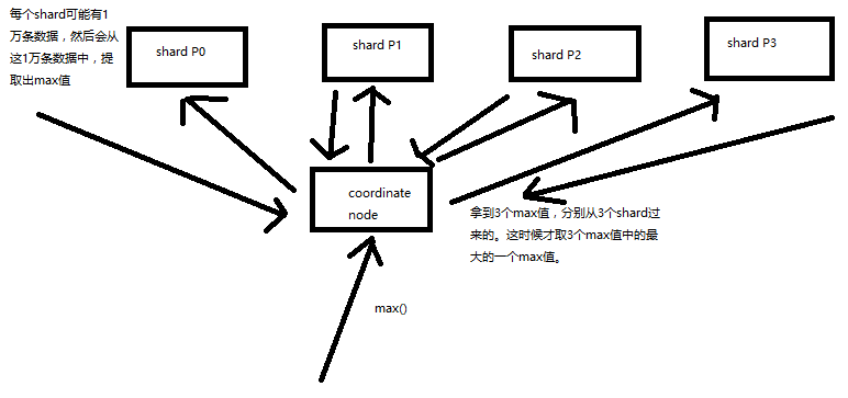
有些聚合分析的算法是不好并行的，比如说 count(distinct)（去重后统计剩余数量，也就是唯一值个数），并不是说在每个 node 上直接就出一些 distinct value 就可以的，因为每个 shard 之间可能还有重复的数据，所以就不准的，这个时候就需要从每个 shard 上把所有相关数据都获取过来，然后计算如下图

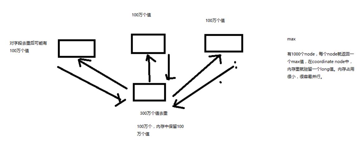
不易并行算法进行聚合的时候，由于数据量可能太大会导致内存占用过多，性能严重影响，甚至内存溢出，这个时候 es 会采取近似聚合的方式，就是采用在每个 node 上进行近估计的方式，得到最终的结论，如：cuont(distcint) 本来是 100 万，可能会返回 105 万，近似估计后的结果，不完全准确，但是速度会很快，一般会达到完全精准的算法的性能的数十倍。

这就会出现一个概念，三角选择原则

三角选择原则

精准 + 实时 + 大数据只能选择 2 个

精准+实时: 没有大数据，数据量很小，那么一般就是单机跑，随便你则么玩儿就可以
精准+大数据：hadoop 批处理，非实时，可以处理海量数据，保证精准，可能会跑几个小时
大数据+实时：es，不精准，近似估计，可能会有百分之几的错误率

近似聚合算法

如果采取近似估计的算法：延时在 100ms 左右，0.5% 错误
如果采取 100% 精准的算法：延时一般在 ns~几十s，甚至几十分钟，几小时， 0% 错误

::: tip 对于这个错误率不知道是怎么出来的，就是一句话数据量非百分百准确 :::

cardinality 去重算法以及每月销售品牌数量统计

cartinality metric 对每个 bucket 中的指定的 field 进行去重，取去重后的 count，类似于 count(distcint)

下面尝试不使用 cartinality 来实现每月销售品牌数量统计

GET /tvs/sales/_search
{
  "size": 0,
  "aggs": {
    "group_by_date": {
      "date_histogram": {
        "field": "sold_date",
        "interval": "month"
      },
      "aggs": {
        "group_by_brand": {
          "terms": {
            "field": "brand"
          }
        }
      }
    }
  }
}

结果返回

{
  "took": 1,
  "timed_out": false,
  "_shards": {
    "total": 5,
    "successful": 5,
    "failed": 0
  },
  "hits": {
    "total": 8,
    "max_score": 0,
    "hits": []
  },
  "aggregations": {
    "group_by_date": {
      "buckets": [
        {
          "key_as_string": "2016-05-01T00:00:00.000Z",
          "key": 1462060800000,
          "doc_count": 1,
          "group_by_brand": {
            "doc_count_error_upper_bound": 0,
            "sum_other_doc_count": 0,
            "buckets": [
              {
                "key": "小米",
                "doc_count": 1
              }
            ]
          }
        },
        {
          "key_as_string": "2016-06-01T00:00:00.000Z",
          "key": 1464739200000,
          "doc_count": 0,
          "group_by_brand": {
            "doc_count_error_upper_bound": 0,
            "sum_other_doc_count": 0,
            "buckets": []
          }
        },
        {
          "key_as_string": "2016-07-01T00:00:00.000Z",
          "key": 1467331200000,
          "doc_count": 1,
          "group_by_brand": {
            "doc_count_error_upper_bound": 0,
            "sum_other_doc_count": 0,
            "buckets": [
              {
                "key": "TCL",
                "doc_count": 1
              }
            ]
          }
        },
        {
          "key_as_string": "2016-08-01T00:00:00.000Z",
          "key": 1470009600000,
          "doc_count": 1,
          "group_by_brand": {
            "doc_count_error_upper_bound": 0,
            "sum_other_doc_count": 0,
            "buckets": [
              {
                "key": "TCL",
                "doc_count": 1
              }
            ]
          }
        },
        {
          "key_as_string": "2016-09-01T00:00:00.000Z",
          "key": 1472688000000,
          "doc_count": 0,
          "group_by_brand": {
            "doc_count_error_upper_bound": 0,
            "sum_other_doc_count": 0,
            "buckets": []
          }
        },
        {
          "key_as_string": "2016-10-01T00:00:00.000Z",
          "key": 1475280000000,
          "doc_count": 1,
          "group_by_brand": {
            "doc_count_error_upper_bound": 0,
            "sum_other_doc_count": 0,
            "buckets": [
              {
                "key": "长虹",
                "doc_count": 1
              }
            ]
          }
        },
        {
          "key_as_string": "2016-11-01T00:00:00.000Z",
          "key": 1477958400000,
          "doc_count": 2,
          "group_by_brand": {
            "doc_count_error_upper_bound": 0,
            "sum_other_doc_count": 0,
            "buckets": [
              {
                "key": "长虹",
                "doc_count": 2
              }
            ]
          }
        },
        {
          "key_as_string": "2016-12-01T00:00:00.000Z",
          "key": 1480550400000,
          "doc_count": 0,
          "group_by_brand": {
            "doc_count_error_upper_bound": 0,
            "sum_other_doc_count": 0,
            "buckets": []
          }
        },
        {
          "key_as_string": "2017-01-01T00:00:00.000Z",
          "key": 1483228800000,
          "doc_count": 1,
          "group_by_brand": {
            "doc_count_error_upper_bound": 0,
            "sum_other_doc_count": 0,
            "buckets": [
              {
                "key": "三星",
                "doc_count": 1
              }
            ]
          }
        },
        {
          "key_as_string": "2017-02-01T00:00:00.000Z",
          "key": 1485907200000,
          "doc_count": 1,
          "group_by_brand": {
            "doc_count_error_upper_bound": 0,
            "sum_other_doc_count": 0,
            "buckets": [
              {
                "key": "小米",
                "doc_count": 1
              }
            ]
          }
        }
      ]
    }
  }
}

可以看到上面的结果，只能统计到每个月的品牌数量，而不是去重的

下面来实现去重后的品牌数量统计

GET /tvs/sales/_search
{
  "size": 0,
  "aggs": {
    "group_by_date": {
      "date_histogram": {
        "field": "sold_date",
        "interval": "month"
      },
      "aggs": {
        "distinct_brand": {
          "cardinality": {
            "field": "brand"
          }
        }
      }
    }
  }
}

返回结果

{
  "took": 6,
  "timed_out": false,
  "_shards": {
    "total": 5,
    "successful": 5,
    "failed": 0
  },
  "hits": {
    "total": 8,
    "max_score": 0,
    "hits": []
  },
  "aggregations": {
    "group_by_date": {
      "buckets": [
        {
          "key_as_string": "2016-05-01T00:00:00.000Z",
          "key": 1462060800000,
          "doc_count": 1,
          "distinct_brand": {
            "value": 1
          }
        },
        {
          "key_as_string": "2016-06-01T00:00:00.000Z",
          "key": 1464739200000,
          "doc_count": 0,
          "distinct_brand": {
            "value": 0
          }
        },
        {
          "key_as_string": "2016-07-01T00:00:00.000Z",
          "key": 1467331200000,
          "doc_count": 1,
          "distinct_brand": {
            "value": 1
          }
        },
        {
          "key_as_string": "2016-08-01T00:00:00.000Z",
          "key": 1470009600000,
          "doc_count": 1,
          "distinct_brand": {
            "value": 1
          }
        },
        {
          "key_as_string": "2016-09-01T00:00:00.000Z",
          "key": 1472688000000,
          "doc_count": 0,
          "distinct_brand": {
            "value": 0
          }
        },
        {
          "key_as_string": "2016-10-01T00:00:00.000Z",
          "key": 1475280000000,
          "doc_count": 1,
          "distinct_brand": {
            "value": 1
          }
        },
        {
          "key_as_string": "2016-11-01T00:00:00.000Z",
          "key": 1477958400000,
          "doc_count": 2,
          "distinct_brand": {
            "value": 1
          }
        },
        {
          "key_as_string": "2016-12-01T00:00:00.000Z",
          "key": 1480550400000,
          "doc_count": 0,
          "distinct_brand": {
            "value": 0
          }
        },
        {
          "key_as_string": "2017-01-01T00:00:00.000Z",
          "key": 1483228800000,
          "doc_count": 1,
          "distinct_brand": {
            "value": 1
          }
        },
        {
          "key_as_string": "2017-02-01T00:00:00.000Z",
          "key": 1485907200000,
          "doc_count": 1,
          "distinct_brand": {
            "value": 1
          }
        }
      ]
    }
  }
}

cardinality 算法内存优化、hll 算法

cardinality 算法内存优化

cardinality 5% 的错误率，性能在 100ms 左右

上面这句话是否是感觉很没有安全感？缺少一些重要的信息，比如是怎么计算来的？那么这会带出来一个配置参数 precision_threshold

GET /tvs/sales/_search
{
    "size" : 0,
    "aggs" : {
        "distinct_brand" : {
            "cardinality" : {
              "field" : "brand",
              "precision_threshold" : 100
            }
        }
    }
}

precision_threshold：在多少个 unique value 以内 cardinality 几乎保证 100% 准确，默认值为 100，它的配置可以优化准确率和内存开销

怎么理解这个 100 个 unique value？

考虑一个场景：brand 去重，如果 brand 的 unique value 在100个以内，比如小米，长虹，三星，TCL，HTL … 在去重后的结果在 100 个以内

cardinality 算法会占用 precision_threshold * 8 byte 内存消耗，100 * 8 = 800 个字节，占用内存很小。而且 unique value 如果的确在值以内，那么可以确保 100% 准确官方给的一个说法是 100，在数百万的 unique value 内错误率在 5% 以内

::: warning 反正我是有点懵逼，解说 precision_threshold 表示的是多少个 unique value ，现在又说官网设置为 100，可以保证数百万 :::

precision_threshold 值设置的越大，占用内存越大，1000 * 8 = 8000 / 1000 = 8KB，可以确保更多 unique value 的场景下 100% 的准确

field 去重 count，这时候 unique value 10000，precision_threshold=10000，10000 * 8 = 80000个byte，80KB

HyperLogLog++（HLL）算法性能优化

cardinality 底层算法：使用 HLL 算法，优化 HLL 算法的性能即可

HLL 会对所有的 uqniue value 取 hash 值，通过 hash 值近似去求 distcint count，所以有一定误差

默认情况下，发送一个 cardinality 请求的时候，会动态地对所有的 field value，取 hash 值;

我们只要将取 hash 值的操作，前移到建立索引的时候，就能优化这个聚合性能了

PUT /tvs/
{
  "mappings": {
    "sales": {
      "properties": {
        "brand": {
          "type": "text",
          "fields": {
            "hash": {
              "type": "murmur3"
            }
          }
        }
      }
    }
  }
}

手动内置 mapping hash 字段

GET /tvs/sales/_search
{
    "size" : 0,
    "aggs" : {
        "distinct_brand" : {
            "cardinality" : {
              "field" : "brand.hash",
              "precision_threshold" : 100
            }
        }
    }
}

percentiles 百分比算法、网站访问时延统计

需求：比如有一个网站，记录下了每次请求的访问的耗时，需要统计 tp50，tp90，tp99

什么是 tp n 呢?

tp50：50% 的请求的耗时最长在多长时间
tp90：90% 的请求的耗时最长在多长时间
tp99：99% 的请求的耗时最长在多长时间

那么可以使用 percentiles 算法

先插入模拟数据

PUT /website
{
    "mappings": {
        "logs": {
            "properties": {
                "latency": {
                    "type": "long"
                },
                "province": {
                    "type": "keyword"
                },
                "timestamp": {
                    "type": "date"
                }
            }
        }
    }
}

POST /website/logs/_bulk
{ "index": {}}
{ "latency" : 105, "province" : "江苏", "timestamp" : "2016-10-28" }
{ "index": {}}
{ "latency" : 83, "province" : "江苏", "timestamp" : "2016-10-29" }
{ "index": {}}
{ "latency" : 92, "province" : "江苏", "timestamp" : "2016-10-29" }
{ "index": {}}
{ "latency" : 112, "province" : "江苏", "timestamp" : "2016-10-28" }
{ "index": {}}
{ "latency" : 68, "province" : "江苏", "timestamp" : "2016-10-28" }
{ "index": {}}
{ "latency" : 76, "province" : "江苏", "timestamp" : "2016-10-29" }
{ "index": {}}
{ "latency" : 101, "province" : "新疆", "timestamp" : "2016-10-28" }
{ "index": {}}
{ "latency" : 275, "province" : "新疆", "timestamp" : "2016-10-29" }
{ "index": {}}
{ "latency" : 166, "province" : "新疆", "timestamp" : "2016-10-29" }
{ "index": {}}
{ "latency" : 654, "province" : "新疆", "timestamp" : "2016-10-28" }
{ "index": {}}
{ "latency" : 389, "province" : "新疆", "timestamp" : "2016-10-28" }
{ "index": {}}
{ "latency" : 302, "province" : "新疆", "timestamp" : "2016-10-29" }

percentiles 用法，下面

GET /website/logs/_search
{
  "size": 0,
  "aggs": {
    "latency_percentiles": {
      "percentiles": {
        "field": "latency",
        "percents": [
          50,
          95,
          99
        ]
      }
    },
    "latency_avg": {
      "avg": {
        "field": "latency"
      }
    }
  }
}

latency_percentiles：所有数据中按百分比计算
latency_avg：所有数据的平均耗时

响应结果如下

{
  "took": 1,
  "timed_out": false,
  "_shards": {
    "total": 5,
    "successful": 5,
    "failed": 0
  },
  "hits": {
    "total": 12,
    "max_score": 0,
    "hits": []
  },
  "aggregations": {
    "latency_avg": {
      "value": 201.91666666666666
    },
    "latency_percentiles": {
      "values": {
        "50.0": 108.5,
        "95.0": 508.24999999999983,
        "99.0": 624.8500000000001
      }
    }
  }
}

至于这个是怎么计算出来的，应该是涉及到数据相关的知识，稍微百度了下，是统计学里面的数据知识

需求：按照省份进行百分比计算

GET /website/logs/_search
{
  "size": 0,
  "aggs": {
    "group_by_province": {
      "terms": {
        "field": "province"
      },
      "aggs": {
        "latency_percentiles": {
          "percentiles": {
            "field": "latency",
            "percents": [
              50,
              95,
              99
            ]
          }
        },
        "latency_avg": {
          "avg": {
            "field": "latency"
          }
        }
      }
    }
  }
}

响应结果

{
  "took": 1,
  "timed_out": false,
  "_shards": {
    "total": 5,
    "successful": 5,
    "failed": 0
  },
  "hits": {
    "total": 12,
    "max_score": 0,
    "hits": []
  },
  "aggregations": {
    "group_by_province": {
      "doc_count_error_upper_bound": 0,
      "sum_other_doc_count": 0,
      "buckets": [
        {
          "key": "新疆",
          "doc_count": 6,
          "latency_avg": {
            "value": 314.5
          },
          "latency_percentiles": {
            "values": {
              "50.0": 288.5,
              "95.0": 587.75,
              "99.0": 640.75
            }
          }
        },
        {
          "key": "江苏",
          "doc_count": 6,
          "latency_avg": {
            "value": 89.33333333333333
          },
          "latency_percentiles": {
            "values": {
              "50.0": 87.5,
              "95.0": 110.25,
              "99.0": 111.65
            }
          }
        }
      ]
    }
  }
}

percentiles rank 以及网站访问时延 SLA 统计

SLA

SLA 就是你提供的服务的标准

我们的网站的提供的访问延时的 SLA，确保所有的请求 100% 都必须在 200ms 以内，大公司内一般都是要求 100% 在 200ms 以内，如果超过 1s，则需要升级到 A 级故障，代表网站的访问性能和用户体验急剧下降

percentiles rank

这个 percentile ranks 其实比 pencentile 还要常用，比如按照品牌分组，计算电视机售价在 1000 占比，2000 占比，3000 占比

需求：在 200ms 以内的，有百分之多少，在 1000 毫秒以内的有百分之多少

GET /website/logs/_search
{
  "size": 0,
  "aggs": {
    "group_by_province": {
      "terms": {
        "field": "province"
      },
      "aggs": {
        "latency_percentile_ranks": {
          "percentile_ranks": {
            "field": "latency",
            "values": [
              200,
              1000
            ]
          }
        }
      }
    }
  }
}

响应结果

{
  "took": 110,
  "timed_out": false,
  "_shards": {
    "total": 5,
    "successful": 5,
    "failed": 0
  },
  "hits": {
    "total": 12,
    "max_score": 0,
    "hits": []
  },
  "aggregations": {
    "group_by_province": {
      "doc_count_error_upper_bound": 0,
      "sum_other_doc_count": 0,
      "buckets": [
        {
          "key": "新疆",
          "doc_count": 6,
          "latency_percentile_ranks": {
            "values": {
              "200.0": 29.40613026819923,
              "1000.0": 100
            }
          }
        },
        {
          "key": "江苏",
          "doc_count": 6,
          "latency_percentile_ranks": {
            "values": {
              "200.0": 100,
              "1000.0": 100
            }
          }
        }
      ]
    }
  }
}

理解这个 200ms 以内和 1000ms 以内：200ms 以内的占总数的百分比？

percentile 的优化

内部使用的是 TDigest 算法，用很多节点来执行百分比的计算，近似估计、有误差，节点越多，越精准

它的配置参数 compression

限制节点数量最多 compression * 20 = 2000 个 node 去计算
默认100
越大，占用内存越多，越精准，性能越差

一个节点占用 32 字节，100 * 20 * 32 = 64KB

如果你想要 percentile 算法越精准，compression 可以设置的越大

基于 doc value 正排索引的聚合内部原理

本章节会开始接待这些疑问：

聚合分析的内部原理是什么？
执行一个聚合操作的时候，内部原理是怎样的呢？
用了什么样的数据结构去执行聚合？
是不是用的倒排索引？

搜索+聚合，写个示例

GET /test_index/test_type/_search
{
	"query": {
		"match": {
			"search_field": "test"
		}
	},
	"aggs": {
		"group_by_agg_field": {
			"terms": {
				"field": "agg_field"
			}
		}
	}
}

基于以上示例来分析：纯用倒排索引来实现的弊端

对于 query 来说，搜索使用倒排索引速度很快

结果出来之后，对于 aggs 来说，如果也使用倒排索引的话就会出现性能低下的问题，以 1000 条数据来说，如果聚合字段是分词的，那么你至少要遍历整个倒排索引数据才能拿到整个 field 的全部值，如果是以正派索引来获取，那么最多遍历 1000 次就能拿到整个 doc 的信息，而往往可能在前面几条就拿到了

所以 es 是使用倒排索引+正排索引（doc value）方式来进行聚合分析操作的

doc value 机制内核级原理深入探秘

对于 doc value，我一直以为就类似于 mysql 表数据一样，基于 id 获取的，但是看这章节并不是，所以看完还是懵逼状态

doc value原理

index-time生成

PUT/POST的时候，就会生成doc value数据，也就是正排索引
核心原理与倒排索引类似

正排索引也会写入磁盘文件中，os cache 先进行缓存以提升访问 doc value 正排索引的性能如果 os cache 内存大小不足够放得下整个正排索引，就会将 doc value 的数据写入磁盘文件中
性能问题：给 jvm 更少内存，64g 服务器给 jvm 最多 16g

es 官方是建议 es 大量是基于 os cache 来进行缓存和提升性能的，不建议用 jvm 内存来进行缓存，那样会导致一定的 gc 开销和 oom 问题，所以给 jvm 更少的内存，给 os cache 更大的内存以 64g 服务器为例，给 jvm 最多 16g，其他的内存给 os cache os cache 可以提升 doc value 和倒排索引的缓存和查询效率

column 压缩

比如以下数据

doc1: 550
doc2: 550
doc3: 500

合并相同值 550，doc1 和 doc2 都保留一个 550 的标识即可

所有值相同，直接保留单值
少于 256 个值，使用 table encoding 模式（一种压缩方式）
大于 256 个值，看有没有最大公约数，有就除以最大公约数，然后保留这个最大公约数

doc1: 36 doc2: 24 6 –> doc1: 6, doc2: 4 –> 保留一个最大公约数 6 的标识，6 也保存起来
如果没有最大公约数，采取 offset 结合压缩的方式：

以上内容，只要明白 doc value 的一个压缩存储，使用层层压缩的方式进行存储的，其他的都太底层了，讲不清

disable doc value

如果的确不需要 doc value，比如不需要聚合等操作，那么可以禁用，减少磁盘空间占用

PUT my_index
{
  "mappings": {
    "my_type": {
      "properties": {
        "my_field": {
          "type": "keyword",
          "doc_values": false
        }
      }
    }
  }
}

string field 聚合实验以及 fielddata 原理初探

本章的知识点需要前面几个章节的知识做铺垫，不然很难看懂是什么

分词的 field 执行 aggs 发现报错

比如有如下数据

PUT /test_index/test_type/1
{
  "test_field": "test"
}

PUT /test_index/test_type/2
{
  "test_field": "test2"
}

使用聚合函数

GET /test_index/test_type/_search
{
  "aggs": {
    "group_by_test_field": {
      "terms": {
        "field": "test_field"
      }
    }
  }
}

发现会报错

{
  "error": {
    "root_cause": [
      {
        "type": "illegal_argument_exception",
        "reason": "Fielddata is disabled on text fields by default. Set fielddata=true on [test_field] in order to load fielddata in memory by uninverting the inverted index. Note that this can however use significant memory."
      }
    ],
    "type": "search_phase_execution_exception",
    "reason": "all shards failed",
    "phase": "query",
    "grouped": true,
    "failed_shards": [
      {
        "shard": 0,
        "index": "test_index",
        "node": "KHsngUpVR5qe_taJBZGTMg",
        "reason": {
          "type": "illegal_argument_exception",
          "reason": "Fielddata is disabled on text fields by default. Set fielddata=true on [test_field] in order to load fielddata in memory by uninverting the inverted index. Note that this can however use significant memory."
        }
      }
    ],
    "caused_by": {
      "type": "illegal_argument_exception",
      "reason": "Fielddata is disabled on text fields by default. Set fielddata=true on [test_field] in order to load fielddata in memory by uninverting the inverted index. Note that this can however use significant memory."
    }
  },
  "status": 400
}

对分词的 field，直接执行聚合操作会报错，大概意思是说，你必须要打开 fielddata，然后将正排索引数据加载到内存中，才可以对分词的 field 执行聚合操作，而且会消耗很大的内存

下面我们按照报错信息来打开 fielddata

配置 fielddata=true

首先查看他默认生成的 mappings

GET /test_index/_mapping/test_type

{
  "test_index": {
    "mappings": {
      "test_type": {
        "properties": {
          "test_field": {
            "type": "text",
            "fields": {
              "keyword": {
                "type": "keyword",
                "ignore_above": 256
              }
            }
          }
        }
      }
    }
  }
}

打开该字段的 fielddata

POST /test_index/_mapping/test_type
{
  "properties": {
    "test_field":{
      "type": "text",
      "fielddata": true
    }
  }
}

查看修改后的 mappings

GET /test_index/_mapping/test_type

{
  "test_index": {
    "mappings": {
      "test_type": {
        "properties": {
          "test_field": {
            "type": "text",
            "fields": {
              "keyword": {
                "type": "keyword",
                "ignore_above": 256
              }
            },
            "fielddata": true
          }
        }
      }
    }
  }
}

然后再次执行前面的聚合分析操作，发现成功了

使用内置 field 不分词，对 string field 进行聚合

对于 text 类型的字段，会默认创建一个 keyword 的内置字段

"test_field": {
  "type": "text",
  "fields": {
    "keyword": {
      "type": "keyword",
      "ignore_above": 256
    }
  }
}

type.keyword：不分词
ignore_above：只截取前 256 个字符存储

那么基于这个特性，可以直接使用这个内置的字段进行聚合操作

GET /test_index/test_type/_search
{
  "size":0,
  "aggs": {
    "group_by_test_field": {
      "terms": {
        "field": "test_field.keyword"
      }
    }
  }
}

分词 field + fielddata 的工作原理

doc value：不分词的所有 field，可以执行聚合操作

如果你的某个 field 不分词，那么在 index-time（索引建立时），就会自动生成 doc value 针对这些不分词的 field 执行聚合操作的时候，自动就会用 doc value 来执行
分词 field，是没有 doc value 的

在 index-time，如果某个 field 是分词的，那么是不会给它建立 doc value 正排索引的因为分词后，占用的空间过于大，所以默认是不支持分词 field 进行聚合的分词 field 默认没有 doc value，所以直接对分词 field 执行聚合操作，是会报错的

对于分词 field，必须打开和使用 fielddata，完全存在于纯内存中。结构和 doc value 类似。如果是 ngram 或者是大量 term，那么必将占用大量的内存。

如果一定要对分词的 field 执行聚合，那么必须将 fielddata=true，然后 es 就会在执行聚合操作的时候，现场将 field 对应的数据，建立一份 fielddata 正排索引，fielddata 正排索引的结构跟 doc value 是类似的，但是只会讲 fielddata 正排索引加载到内存中来，然后基于内存中的 fielddata 正排索引执行分词 field 的聚合操作

如果直接对分词 field 执行聚合，会报错，才会让我们开启 fielddata=true，告诉我们，会将 fielddata uninverted index，正排索引，加载到内存，会耗费内存空间

为什么 fielddata 必须在内存？因为大家自己思考一下，分词的字符串，需要按照 term 进行聚合，需要执行更加复杂的算法和操作，如果基于磁盘和 os cache 那么性能会很差

fielddata 内存控制以及 circuit breaker 短路器

fielddata 核心原理

fielddata 加载到内存的过程是 lazy 加载的，对一个 analzyed field 执行聚合时，才会加载，而且是 field-level（字段级别而不是该 doc 的所有字段）加载的，一个 index 的一个 field，所有 doc 都会被加载而不是少数 doc，不是 index-time 创建，是 query-time 创建

fielddata 内存限制

有一个配置字段可以配置 indices.fielddata.cache.size: 20%，

作用是占用的内存超出了这个比例的限制，清除内存已有 fielddata 数据，默认无限制。

虽然可以限制内存使用，但是会导致频繁 evict 和 reload，大量 IO 性能损耗，以及内存碎片和 gc

配置方式：在配置文件 elasticsearch-5.2.0/config/elasticsearch.yml 新增该配置参数即可

::: tip 该配置文件中默认是没有改参数配置的，所以搜不到该配置的关键信息 :::

监控 fielddata 内存使用

// 所有分片的统计信息
GET /_stats/fielddata?fields=*

// 获取每个 node 的占用信息
GET /_nodes/stats/indices/fielddata?fields=*

// 获取每个 node 的每个索引占用信息
GET /_nodes/stats/indices/fielddata?level=indices&fields=*

circuit breaker

如果一次 query load 的 feilddata 超过总内存，就会 oom 内存溢出

circuit breaker 会估算 query 要加载的 fielddata 大小，如果超出总内存就短路，query 直接失败

indices.breaker.fielddata.limit：fielddata 的内存限制，默认 60%
indices.breaker.request.limit：执行聚合的内存限制，默认 40%
indices.breaker.total.limit：综合上面两个，限制在 70% 以内

这些属性也是在 elasticsearch.yml 中配置的

fielddata filter 的细粒度内存加载控制

可以通过 mappings 来定制每个 fielddata 的内存使用

POST /test_index/_mapping/my_type
{
  "properties": {
    "my_field": {
      "type": "text",
      "fielddata": {
        "filter": {
          "frequency": {
            "min":              0.01,
            "min_segment_size": 500  
          }
        }
      }
    }
  }
}

min：仅仅加载至少在 1% 的 doc 中出现过的 term 对应的 fielddata

比如说总共有 1000 个 doc，hello 这个值必须在 10 个 doc 中出现，那么这个 hello 对应的 fielddata 才会加载到内存中来
min_segment_size：少于 500 doc 的 segment 不加载 fielddata

加载 fielddata 的时候，也是按照 segment 去进行加载的，某个 segment 里面的 doc 数量少于 500 个，那么这个 segment 的 fielddata 就不加载

这个，就我的经验来看，有点底层了，一般不会去设置它，大家知道就好

fielddata 预加载机制以及序号标记预加载

如果真的要对分词的 field 执行聚合，那么每次都在 query-time 现场生成 fielddata 并加载到内存中来，速度可能会比较慢

我们是不是可以预先生成加载 fielddata 到内存中来？

fielddata 预加载

POST /test_index/_mapping/test_type
{
  "properties": {
    "test_field": {
      "type": "string",
      "fielddata": {
        "loading" : "eager"
      }
    }
  }
}

上面的配置可以将 query-time 的 fielddata 生成和加载到内存，变为 index-time，建立倒排索引的时候，会同步生成 fielddata 并且加载到内存中来，这样的话，对分词 field 的聚合性能当然会大幅度增强

序号标记预加载

global ordinal 原理解释

有如下值，右侧表示 doc 的某一个字段内容

doc1: status1
doc2: status2
doc3: status2
doc4: status1

有很多重复值的情况，会进行 global ordinal 标记，可以理解为享元模式，标记后的示意图如下

status1 --> 0
status2 --> 1

doc1: 0
doc2: 1
doc3: 1
doc4: 0

建立的 fielddata 也会是这个样子的，这样的好处就是减少重复字符串的出现的次数，减少内存的消耗

配置语法如下

POST /test_index/_mapping/test_type
{
  "properties": {
    "test_field": {
      "type": "string",
      "fielddata": {
        "loading" : "eager_global_ordinals"
      }
    }
  }
}

海量 bucket 优化机制：从深度优先到广度优先

本章讲解当 buckets 数量特别多的时候，深度优先和广度优先的原理

场景定义，我们的数据：是每个演员的每个电影的评论

每个演员的评论的数量、每个演员的每个电影的评论的数量

评论数量排名前 10 个的演员、每个演员的电影取到评论数量排名前 5 的电影

{
  "aggs" : {
    "actors" : {
      "terms" : {
         "field" :        "actors",
         "size" :         10,
         "collect_mode" : "breadth_first"
      },
      "aggs" : {
        "costars" : {
          "terms" : {
            "field" : "films",
            "size" :  5
          }
        }
      }
    }
  }
}

collect_mode：默认是深度优先的方式去执行聚合操作的，可以修改为广度优先

对于深度和广度优先的解释，在这个场景中，你要记得数据是「是每个演员的每个电影的评论」。

深度优先

假设 100 个演员，只需要 10 个，在这个场景中，会优先构建完成一颗树
```
actor1            actor2            .... actor
film1 film2 film3   film1 film2 film3   ...film
```
100 * 平均每个演员有 10 步骤电影 = 1000
广度优先

先不管电影，先构建 100 个演员的数据，截取前 10 个，然后在 10 个中构建电影数据，最后只取 5 个电影数据 100 -> 10，10 & 10 = 100

从构建的数据量来看，广度优先胡更节约内存，1000/100=10 10 倍的差距

关系型与 document 类型数据模型对比

本章对关系型和 document 类型数据模型进行一个简单的介绍

关系型数据库的数据模型

比如有如下两个实体

public class Department {

	private Integer deptId;
	private String name;
	private String desc;
	private List<Employee> employees;

}

public class Employee {

	private Integer empId;
	private String name;
	private Integer age;
	private String gender;
	private Department dept;

}

对应关系型数据库中

department表

dept_id
name
desc

employee表

emp_id
name
age
gender
dept_id

三范式 –> 将每个数据实体拆分为一个独立的数据表，同时使用主外键关联关系将多个数据表关联起来 –> 确保没有任何冗余的数据

一份数据，只会放在一个数据表中，要想查看某个员工的部门，需要到另外一个表中查询

es 文档数据模型

{
	"deptId": "1",
	"name": "研发部门",
	"desc": "负责公司的所有研发项目",
	"employees": [
		{
			"empId": "1",
			"name": "张三",
			"age": 28,
			"gender": "男"
		},
		{
			"empId": "2",
			"name": "王兰",
			"age": 25,
			"gender": "女"
		},
		{
			"empId": "3",
			"name": "李四",
			"age": 34,
			"gender": "男"
		}
	]
}

es 更加类似于面向对象的数据模型，将所有由关联关系的数据，放在一个 doc json 类型数据中，整个数据的关系，还有完整的数据，都放在了一起

总结

关系型数据库：提倡不冗余数据，数据分离
文档型数据：相关联的数据放在一起，一定的冗余数据
通过应用层 join 实现用户与博客的关联

案例介绍

案例背景：博客网站，我们会模拟各种用户发表各种博客，然后针对用户和博客之间的关系进行数据建模，同时针对建模好的数据执行各种搜索/聚合的操作

先使用关系型的思维来构造数据：在构造数据模型的时候，还是将有关联关系的数据，然后分割为不同的实体，类似于关系型数据库中的模型

构造用户与博客数据

PUT /website/users/1
{
  "name": "小鱼儿",
  "email": "xiaoyuer@sina.com",
  "birthday": "1980-01-01"
}

PUT /website/blogs/1
{
  "title": "我的第一篇博客",
  "content": "这是我的第一篇博客，开通啦！！！",
  "userId": 1
}

一个用户对应多个博客，一对多的关系，做了建模，建模方式为分割实体，类似三范式的方式，用主外键关联关系，将多个实体关联起来

join 查询

需求：搜索到小鱼儿的所有博客

先搜索到小鱼儿的 userId

GET /website/users/_search
{
  "query": {
    "term": {
      "name.keyword": "小鱼儿"
    }
  }
}

{
  "took": 129,
  "timed_out": false,
  "_shards": {
    "total": 5,
    "successful": 5,
    "failed": 0
  },
  "hits": {
    "total": 1,
    "max_score": 0.2876821,
    "hits": [
      {
        "_index": "website",
        "_type": "users",
        "_id": "1",
        "_score": 0.2876821,
        "_source": {
          "name": "小鱼儿",
          "email": "xiaoyuer@sina.com",
          "birthday": "1980-01-01"
        }
      }
    ]
  }
}

再根据 userId 搜索小鱼儿的所有博客

GET /website/blogs/_search
{
  "query": {
    "constant_score": {
      "filter": {
        "term": {
          "userId": 1
        }
      }
    }
  }
}

{
  "took": 2,
  "timed_out": false,
  "_shards": {
    "total": 5,
    "successful": 5,
    "failed": 0
  },
  "hits": {
    "total": 1,
    "max_score": 1,
    "hits": [
      {
        "_index": "website",
        "_type": "blogs",
        "_id": "1",
        "_score": 1,
        "_source": {
          "title": "我的第一篇博客",
          "content": "这是我的第一篇博客，开通啦！！！",
          "userId": 1
        }
      }
    ]
  }
}

上面的操作，就属于应用层的 join，在应用层先查出一份数据，然后再查出一份数据，进行关联;

试想一下，如果是批量查询，那么需要返回第一次的结果，然后再拿这一大批数据去搜索，性能上相对来说有点差了

关系型模型的优缺点

优点：数据不冗余，维护方便
缺点：应用层 join，如果关联数据过多，导致查询过大，性能很差
通过数据冗余实现用户与博客的关联

第二种建模方式：用冗余数据，采用文档数据模型，进行数据建模，实现用户和博客的关联

冗余数据，就是说，将可能会进行搜索的条件和要搜索的数据，放在一个 doc 中

构造用户与博客数据

DELETE website

PUT /website/users/1
{
  "name": "小鱼儿",
  "email": "xiaoyuer@sina.com",
  "birthday": "1980-01-01"
}

PUT /website/blogs/1
{
  "title": "我的第一篇博客",
  "content": "这是我的第一篇博客，开通啦！！！",
  "userInfo": {
    "userId": 1,
    "username": "小鱼儿"
  }
}

join 查询

搜索数据，需求：还是前面的需求，查找小鱼儿的所有博客

GET /website/blogs/_search
{
  "query": {
    "constant_score": {
      "filter": {
        "term": {
          "userInfo.username.keyword": "小鱼儿"
        }
      }
    }
  }
}

{
  "took": 2,
  "timed_out": false,
  "_shards": {
    "total": 5,
    "successful": 5,
    "failed": 0
  },
  "hits": {
    "total": 1,
    "max_score": 1.2,
    "hits": [
      {
        "_index": "website",
        "_type": "blogs",
        "_id": "1",
        "_score": 1.2,
        "_source": {
          "title": "我的第一篇博客",
          "content": "这是我的第一篇博客，开通啦！！！",
          "userInfo": {
            "userId": 1,
            "username": "小鱼儿"
          }
        }
      }
    ]
  }
}

现在就不需要走应用层的 join：先搜一个数据，找到 id，再去搜另一份数据，直接走一个有冗余数据的 type 即可，指定要的搜索条件，即可搜索出自己想要的数据来

文档型模型的优缺点

优点：性能高，不需要执行两次搜索
缺点：数据冗余，维护成本高

每次如果你的 username 变化了，同时要更新 user type 和 blog type

一般来说，对于 es 这种 NoSQL 类型的数据存储来讲，都是冗余模式，当然，你要去维护数据的关联关系，也是很有必要的，所以一旦出现冗余数据的修改，必须记得将所有关联的数据全部更新

对每个用户发表的博客进行分组

构造数据

要分组的话，我们来构造更多的数据

PUT /website/users/2
{
  "name": "花无缺 ",
  "email": "huawuque@sina.com",
  "birthday": "1960-01-01"
}

PUT /website/blogs/2
{
  "title": "我是花无缺",
  "content": "这是我的第一篇博客，开通啦！！！",
  "userInfo": {
    "userId": 2,
    "username": "花无缺"
  }
}

PUT /website/users/3
{
  "name": "黄药师",
  "email": "huangyaoshi@sina.com",
  "birthday": "1970-10-24"
}

PUT /website/blogs/3
{
  "title": "我是黄药师",
  "content": "我是黄药师啊，各位同学们！！！",
  "userInfo": {
    "userId": 1,
    "username": "黄药师"
  }
}

对每个用户发表的博客进行分组

需求：按用户名进行博客的分组统计

GET /website/blogs/_search
{
  "size": 0,
  "aggs": {
    "group_by_username": {
      "terms": {
        "field": "userInfo.username.keyword"
      },
      "aggs": {
        "top_blogs": {
          "top_hits": {
            "_source": {
              "include": ["title"]
            },
            "size": 10
          }
        }
      }
    }
  }
}


{
  "took": 2,
  "timed_out": false,
  "_shards": {
    "total": 5,
    "successful": 5,
    "failed": 0
  },
  "hits": {
    "total": 3,
    "max_score": 0,
    "hits": []
  },
  "aggregations": {
    "group_by_username": {
      "doc_count_error_upper_bound": 0,
      "sum_other_doc_count": 0,
      "buckets": [
        {
          "key": "小鱼儿",
          "doc_count": 1,
          "top_blogs": {
            "hits": {
              "total": 1,
              "max_score": 1,
              "hits": [
                {
                  "_index": "website",
                  "_type": "blogs",
                  "_id": "1",
                  "_score": 1,
                  "_source": {
                    "title": "我的第一篇博客"
                  }
                }
              ]
            }
          }
        },
        {
          "key": "花无缺",
          "doc_count": 1,
          "top_blogs": {
            "hits": {
              "total": 1,
              "max_score": 1,
              "hits": [
                {
                  "_index": "website",
                  "_type": "blogs",
                  "_id": "2",
                  "_score": 1,
                  "_source": {
                    "title": "我是花无缺"
                  }
                }
              ]
            }
          }
        },
        {
          "key": "黄药师",
          "doc_count": 1,
          "top_blogs": {
            "hits": {
              "total": 1,
              "max_score": 1,
              "hits": [
                {
                  "_index": "website",
                  "_type": "blogs",
                  "_id": "3",
                  "_score": 1,
                  "_source": {
                    "title": "我是黄药师"
                  }
                }
              ]
            }
          }
        }
      ]
    }
  }
}

可以看到不需要再应用中 join 了，直接查询出来

对文件系统进行数据建模以及文件搜索实战

本章主要讲解对文件路径的存储于搜索

path_hierarchy analyzer

这个分词的作用是什么呢？直接看一个分词例子即可知道

GET /_analyze
{
  "text": "H:/dev/note/note-book",
  "tokenizer": "path_hierarchy"
}


{
  "tokens": [
    {
      "token": "H:",
      "start_offset": 0,
      "end_offset": 2,
      "type": "word",
      "position": 0
    },
    {
      "token": "H:/dev",
      "start_offset": 0,
      "end_offset": 6,
      "type": "word",
      "position": 0
    },
    {
      "token": "H:/dev/note",
      "start_offset": 0,
      "end_offset": 11,
      "type": "word",
      "position": 0
    },
    {
      "token": "H:/dev/note/note-book",
      "start_offset": 0,
      "end_offset": 21,
      "type": "word",
      "position": 0
    }
  ]
}

数据构造

先 mappings，

fs: filesystem

PUT /fs
{
  "settings": {
    "analysis": {
      "analyzer": {
        "paths":{
          "tokenizer": "path_hierarchy"
        }
      }
    }
  }
}

PUT /fs/_mapping/file
{
  "properties": {
    "name": {
      "type":  "keyword"
    },
    "path": {
      "type":  "keyword",
      "fields": {
        "tree": {
          "type":     "text",
          "analyzer": "paths"
        }
      }
    }
  }
}

插入数据

PUT /fs/file/1
{
  "name":     "README.txt",
  "path":     "/workspace/projects/helloworld",
  "contents": "这是我的第一个 elasticsearch 程序"
}

搜索数据

需求：搜索文件内容包含 elasticsearch，且在 /workspace/projects 下的文件

GET /fs/file/_search
{
  "query": {
   "bool": {
     "must": [
       {"match": {
         "contents": "elasticsearch"
       }}
     ],
     "filter": {
       "term": {
         "path.tree": "/workspace/projects"
       }
     }
   }
  }
}

GET /fs/file/_search
{
  "query": {
    "bool": {
      "must": [
        {"match": {
           "contents": "elasticsearch"
        }},
        {
          "constant_score": {
            "filter": {
              "term": {
                "path.tree": "/workspace/projects"
              }
            }
          }
        }
      ]
    }
  }
}

上面是两种 filter 的用法，实现结果一致，不同的只是评分结果不一致

{
  "took": 2,
  "timed_out": false,
  "_shards": {
    "total": 5,
    "successful": 5,
    "failed": 0
  },
  "hits": {
    "total": 1,
    "max_score": 1.284885,
    "hits": [
      {
        "_index": "fs",
        "_type": "file",
        "_id": "1",
        "_score": 1.284885,
        "_source": {
          "name": "README.txt",
          "path": "/workspace/projects/helloworld",
          "contents": "这是我的第一个 elasticsearch 程序"
        }
      }
    ]
  }
}

基于全局锁实现悲观锁并发控制

悲观锁介绍

之前讲解了基于 version 的乐观锁并发控制

在数据建模章节，结合文件系统建模的这个案例，把悲观锁的并发控制，3 种锁粒度都给大家仔细讲解一下

本章讲解：最粗的一个粒度，全局锁

考虑一个场景：多个线程，并发地给 /workspace/projects/helloworld 下的 README.txt 修改文件名

乐观锁：
1. get current version
2. 带着这个 current version 去执行修改，如果一旦发现数据已经被别人给修改了， version 号跟之前自己获取的已经不一样了; 那么必须重新获取新的 version 号再次尝试修改
悲观锁
1. 上来就先加锁
2. 此时就只有你一个能对这数据进行修改

全局锁

第一种锁，全局锁：直接锁掉整个 fs index

::: tip 在应用中，利用 _create 语法，创建空的 doc ，让 es 保证只能有一个被创建成功的思路 :::

PUT /fs/lock/global/_create
{}

fs: 你要上锁的那个 index
lock: 就是你指定的一个对这个 index 上全局锁的一个 type
global: 就是你上的全局锁对应的这个 doc 的 id
_create：强制必须是创建，如果 /fs/lock/global 这个 doc 已经存在，那么创建失败，报错

利用了 doc 来进行上锁 /fs/lock/global /index/type/id --> doc

重复执行该创建语法就会报错，那么没有抢占到锁的线程需要重复此操作

{
  "error": {
    "root_cause": [
      {
        "type": "version_conflict_engine_exception",
        "reason": "[lock][global]: version conflict, document already exists (current version [1])",
        "index_uuid": "IYbj0OLGQHmMUpLfbhD4Hw",
        "shard": "2",
        "index": "fs"
      }
    ],
    "type": "version_conflict_engine_exception",
    "reason": "[lock][global]: version conflict, document already exists (current version [1])",
    "index_uuid": "IYbj0OLGQHmMUpLfbhD4Hw",
    "shard": "2",
    "index": "fs"
  },
  "status": 409
}

抢占到该锁的线程，就可以执行各种操作了，比如完成上面的需求，修改文件名称

POST /fs/file/1/_update
{
  "doc": {
    "name": "README-update.txt"
  }
}

操作完成后，释放当前的锁，也就是删除那个空的 doc

DELETE /fs/lock/global

这个时候，另外一个线程就会创建成功，然后执行它自己的逻辑

全局锁的优点和缺点

优点：操作非常简单，非常容易使用，成本低
缺点：你直接就把整个 index 给上锁了，这个时候对 index 中所有的 doc 的操作，都会被 block 住，导致整个系统的并发能力很低

::: warning 这里只是利用了另外一个 type 来创建空的 doc，这样应该是一条 doc 吧？怎么说是整个 index 呢？难道意思是说所有的使用都是用这一个 doc？ /fs/lock/global

如果所有的都用这一个 doc 的话，那么的确的全局的 :::

什么时候使用？上锁解锁的操作不是频繁，每次上锁之后，执行的操作的耗时不会太长

基于 document 锁实现悲观锁并发控制

全局锁一次性就锁整个 index，对这个 index 的所有增删改操作都会被 block 住，如果上锁不频繁，还可以，比较简单

细粒度的一个锁：document 锁，每次只对你要操作的 doc 进行上锁。不影响其他 doc

document 锁的思路，是用脚本进行上锁，如下

POST /fs/lock/1/_update
{
  "upsert": { "process_id": 123 },
  "script": {
     "lang": "groovy",
     "inline": "if ( ctx._source.process_id != process_id ) { assert false }; ctx.op = 'noop';",        "params": {
       "process_id": 123
     }
  }
}

upsert：指定的 doc 不存在的时候使用该内容初始化 doc
script：指定的 doc 存在的时候使用该脚本
params：script 中可以使用
process_id：

充当一个唯一标识，比如：某个服务实例 ID + 当前操作的线程 ID 组成一个唯一标识
assert false，不是当前进程加锁的话，则抛出异常
ctx.op=’noop’，不做任何修改

::: tip 这里需要传入参数，会导致 es 识别脚本语言有误，所以这里需要明确协商 groovy；同时，inline 默认是禁止的，之前讲过用文件方式，文件方式是默认支持的

开启 inline 需要在 elasticsearch.yml 配置文件中增加属性 script.inline: on

完成之后需要重启 es :::

当 process_id 相等的时候返回的数据如下

{
  "_index": "fs",
  "_type": "lock",
  "_id": "1",
  "_version": 3,
  "result": "noop",
  "_shards": {
    "total": 0,
    "successful": 0,
    "failed": 0
  }
}

当 process_id 不相等的时候返回的数据如下

{
  "error": {
    "root_cause": [
      {
        "type": "remote_transport_exception",
        "reason": "[KHsngUp][127.0.0.1:9300][indices:data/write/update[s]]"
      }
    ],
    "type": "illegal_argument_exception",
    "reason": "failed to execute script",
    "caused_by": {
      "type": "script_exception",
      "reason": "error evaluating if ( ctx._source.process_id != process_id ) { assert false }; ctx.op = 'noop';",
      "caused_by": {
        "type": "power_assertion_error",
        "reason": "assert false\n"
      },
      "script_stack": [],
      "script": "",
      "lang": "groovy"
    }
  },
  "status": 400
}

还可以执行下 refresh 加速生效

POST /fs/_refresh

加锁成之后就可以处理自己的业务操作了。处理完成之后释放锁

DELETE /fs/lock/1

或者使用批量语法解锁

PUT /fs/lock/_bulk
{ "delete": { "_id": 1}}

基于共享锁和排他锁实现悲观锁并发控制

读写锁概念

共享锁：所有线程都可获得该锁，用于读取数据
排他锁：只能有一个线程获得该锁，用于写数据

共享锁和排他锁的作用是读写分离，但是共享锁和排他锁是互斥的：

有共享锁则排他锁不能被获取
有排他锁则共享锁不能被获取

简单说就是读写操作只能存在一种

::: tip 在我的认知里面读写分离，是为了解决写数据并发竞争，提高读并发性能，因为适合于读大于写的场景；

但是有一个问题，有可能一直不释放造成写饥饿？ :::

下面来实现读写锁实验

共享锁/读锁获取

POST /fs/lock/1/_update
{
  "upsert": {
    "lock_type": "shared",
    "lock_count": 1
  },
  "script": {
     "lang": "groovy",
     "inline": "if ( ctx._source.lock_type == 'exclusive' ) { assert false }; ctx._source.lock_count++;"
  }
}

多次获取共享锁结果
{
  "_index": "fs",
  "_type": "lock",
  "_id": "1",
  "_version": 6,
  "found": true,
  "_source": {
    "lock_type": "shared",
    "lock_count": 2
  }
}

lock_type：shared 共享锁/读锁、exclusive 排他锁/写锁
lock_count：锁持有数量，用于共享锁的统计
script：当时共享锁的时候，将 lock_count 自增 1

获取排他锁

利用 create 语法来创建，当该 doc 存在的时候，就会报错

PUT /fs/lock/1/_create
{ "lock_type": "exclusive" }

报错如下
{
  "error": {
    "root_cause": [
      {
        "type": "version_conflict_engine_exception",
        "reason": "[lock][1]: version conflict, document already exists (current version [6])",
        "index_uuid": "ksKH094bQQuh7PaGY8Jb7w",
        "shard": "3",
        "index": "fs"
      }
    ],
    "type": "version_conflict_engine_exception",
    "reason": "[lock][1]: version conflict, document already exists (current version [6])",
    "index_uuid": "ksKH094bQQuh7PaGY8Jb7w",
    "shard": "3",
    "index": "fs"
  },
  "status": 409
}

有共享锁在的话，就需要读线程在操作完成之后释放自己的共享锁

释放共享锁

每次执行该操作，就将锁数量自减 1，当等于 0 的时候就删除自己。这样排他锁就能上锁成功了

POST /fs/lock/1/_update
{
  "script": "if(--ctx._source.lock_count == 0){ ctx.op = 'delete'}"
}

被删除时返回的数据：result=deleted

{
  "_index": "fs",
  "_type": "lock",
  "_id": "1",
  "_version": 8,
  "result": "deleted",
  "_shards": {
    "total": 2,
    "successful": 1,
    "failed": 0
  }
}

释放排他锁

通过删除 doc 来达到释放

DELETE /fs/lock/1

小结

以自己的观点来看，都是利用了 es 的 doc 创建报错语法和脚本判定等语法来保证数据的竞争上锁的。

基于 nested object 实现博客与评论嵌套关系

之前冗余数据方式的来建模，其实用的就是 object 类型，我们这里又要引入一种新的 object 类型：nested object 类型

会使用 object 类型来实现一个需求：搜索 28 岁的黄药师的评论，然后引出为什么需要使用 nested objec 类型

object 类型

删除 website index
插入模拟数据
查看自动生成的 mappings

DELETE /website

PUT /website/blogs/6
{
  "title": "花无缺发表的一篇帖子",
  "content":  "我是花无缺，大家要不要考虑一下投资房产和买股票的事情啊。。。",
  "tags":  [ "投资", "理财" ],
  "comments": [
    {
      "name":    "小鱼儿",
      "comment": "什么股票啊？推荐一下呗",
      "age":     28,
      "stars":   4,
      "date":    "2016-09-01"
    },
    {
      "name":    "黄药师",
      "comment": "我喜欢投资房产，风，险大收益也大",
      "age":     31,
      "stars":   5,
      "date":    "2016-10-22"
    }
  ]
}

GET /website/blogs/_mapping

{
  "website": {
    "mappings": {
      "blogs": {
        "properties": {
          "comments": {
            "properties": {
              "age": {
                "type": "long"
              },
              "comment": {
                "type": "text",
                "fields": {
                  "keyword": {
                    "type": "keyword",
                    "ignore_above": 256
                  }
                }
              },
              "date": {
                "type": "date"
              },
              "name": {
                "type": "text",
                "fields": {
                  "keyword": {
                    "type": "keyword",
                    "ignore_above": 256
                  }
                }
              },
              "stars": {
                "type": "long"
              }
            }
          },
          "content": {
            "type": "text",
            "fields": {
              "keyword": {
                "type": "keyword",
                "ignore_above": 256
              }
            }
          },
          "tags": {
            "type": "text",
            "fields": {
              "keyword": {
                "type": "keyword",
                "ignore_above": 256
              }
            }
          },
          "title": {
            "type": "text",
            "fields": {
              "keyword": {
                "type": "keyword",
                "ignore_above": 256
              }
            }
          }
        }
      }
    }
  }
}

实现搜索需求

GET /website/blogs/_search
{
  "query": {
    "bool": {
      "must": [
        {
          "match": {
            "comments.name":"黄药师"
          }
        },{
          "match": {
            "comments.age":28
          }
        }
      ]
    }
  }
}

搜索的结果是，id=6 这条数据被查询出来了，结果又一点不太对，被查询出来的结果中黄药师的年龄是 31

这个就涉及到了 object 类型的底层存储结构

{
  "title":            [ "花无缺", "发表", "一篇", "帖子" ],
  "content":          [ "我", "是", "花无缺", "大家", "要不要", "考虑", "一下", "投资", "房产", "买", "股票", "事情" ],
  "tags":             [ "投资", "理财" ],
  "comments.name":    [ "小鱼儿", "黄药师" ],
  "comments.comment": [ "什么", "股票", "推荐", "我", "喜欢", "投资", "房产", "风险", "收益", "大" ],
  "comments.age":     [ 28, 31 ],
  "comments.stars":   [ 4, 5 ],
  "comments.date":    [ "2016-09-01", "2016-10-22"]
}

object 类型底层数据结构，会将一个 json 数组中的数据，进行扁平化，所以，直接命中了这个 document，name=黄药师，age=28，正好符合

nested objec 类型

这次我们改用 nested objec 类型

DELETE /website

PUT /website
{
  "mappings": {
    "blogs": {
      "properties": {
        "comments": {
          "type": "nested",
          "properties": {
            "name":    { "type": "string"  },
            "comment": { "type": "string"  },
            "age":     { "type": "short"   },
            "stars":   { "type": "short"   },
            "date":    { "type": "date"    }
          }
        }
      }
    }
  }
}

GET /website/blogs/_mapping

{
  "website": {
    "mappings": {
      "blogs": {
        "properties": {
          "comments": {
            "type": "nested",
            "properties": {
              "age": {
                "type": "short"
              },
              "comment": {
                "type": "text"
              },
              "date": {
                "type": "date"
              },
              "name": {
                "type": "text"
              },
              "stars": {
                "type": "short"
              }
            }
          },
          "content": {
            "type": "text",
            "fields": {
              "keyword": {
                "type": "keyword",
                "ignore_above": 256
              }
            }
          },
          "tags": {
            "type": "text",
            "fields": {
              "keyword": {
                "type": "keyword",
                "ignore_above": 256
              }
            }
          },
          "title": {
            "type": "text",
            "fields": {
              "keyword": {
                "type": "keyword",
                "ignore_above": 256
              }
            }
          }
        }
      }
    }
  }
}

对比 mapping 发现，comments 多了一个 "type": "nested"

这次再查询就会发现搜索不到这一条数据了，成功了。

注意查询使用的类型也是 nested

GET /website/blogs/_search
{
  "query": {
    "nested": {
      "path": "comments",
      "score_mode": "none",
      "query": {
        "bool": {
          "must": [
            {
              "match": {
                "comments.name":"黄药师"
              }
            },{
              "match": {
                "comments.age":28
              }
            }
          ]
        }
      }
    }
  }
}

score_mode：分数计算模式，none 为不评分

这个时候底层存储数据其实就类似关联表那样的数据结构了

{
  "comments.name":    [ "小鱼儿" ],
  "comments.comment": [ "什么", "股票", "推荐" ],
  "comments.age":     [ 28 ],
  "comments.stars":   [ 4 ],
  "comments.date":    [ 2014-09-01 ]
}
{
  "comments.name":    [ "黄药师" ],
  "comments.comment": [ "我", "喜欢", "投资", "房产", "风险", "收益", "大" ],
  "comments.age":     [ 31 ],
  "comments.stars":   [ 5 ],
  "comments.date":    [ 2014-10-22 ]
}
{
  "title":            [ "花无缺", "发表", "一篇", "帖子" ],
  "body":             [ "我", "是", "花无缺", "大家", "要不要", "考虑", "一下", "投资", "房产", "买", "股票", "事情" ],
  "tags":             [ "投资", "理财" ]
}

nested object 聚合分析

分析每个月的评论的评分的平均值

需求分析：

每个月的评论
评论的平均值

GET /website/blogs/_search
{
  "size": 0,
  "aggs": {
    "comments_nested": {
      "nested": {
        "path": "comments"
      },
      "aggs": {
        "group_by_month": {
          "date_histogram": {
            "field": "comments.date",
            "interval": "month",
            "format": "yyyy-MM"
          },
          "aggs":{
            "ave_stars":{
              "avg": {
                "field": "comments.stars"
              }
            }
          }
        }
      }
    }
  }
}

响应结果

{
  "took": 1,
  "timed_out": false,
  "_shards": {
    "total": 5,
    "successful": 5,
    "failed": 0
  },
  "hits": {
    "total": 1,
    "max_score": 0,
    "hits": []
  },
  "aggregations": {
    "comments_nested": {
      "doc_count": 2,
      "group_by_month": {
        "buckets": [
          {
            "key_as_string": "2016-09",
            "key": 1472688000000,
            "doc_count": 1,
            "ave_stars": {
              "value": 4
            }
          },
          {
            "key_as_string": "2016-10",
            "key": 1475280000000,
            "doc_count": 1,
            "ave_stars": {
              "value": 5
            }
          }
        ]
      }
    }
  }
}

统计每 10 岁一个年龄段的评论，文章标签个数

需求分析：

按 10 岁一个年龄段分组
下钻分析：这些评论的文章标签分组

GET /website/blogs/_search
{
  "size": 0,
  "aggs": {
    "comments_nested": {
      "nested": {
        "path": "comments"
      },
      "aggs": {
         "group_by_age": {
            "histogram": {
              "field": "comments.age",
              "interval": 10
            },
            "aggs": {
              "group_by_tags": {
                "terms": {
                  "field": "tags.keyword"
                }
              }
            }
          }
      }
    }
  }
}

{
  "took": 38,
  "timed_out": false,
  "_shards": {
    "total": 5,
    "successful": 5,
    "failed": 0
  },
  "hits": {
    "total": 1,
    "max_score": 0,
    "hits": []
  },
  "aggregations": {
    "comments_nested": {
      "doc_count": 2,
      "group_by_age": {
        "buckets": [
          {
            "key": 20,
            "doc_count": 1,
            "group_by_tags": {
              "doc_count_error_upper_bound": 0,
              "sum_other_doc_count": 0,
              "buckets": []
            }
          },
          {
            "key": 30,
            "doc_count": 1,
            "group_by_tags": {
              "doc_count_error_upper_bound": 0,
              "sum_other_doc_count": 0,
              "buckets": []
            }
          }
        ]
      }
    }
  }
}

可见统计分析失败了。这个是因为在 nested 中的时候需要引用外部的字段需要额外的配置 reverse_nested

GET /website/blogs/_search
{
  "size": 0,
  "aggs": {
    "comments_nested": {
      "nested": {
        "path": "comments"
      },
      "aggs": {
         "group_by_age": {
            "histogram": {
              "field": "comments.age",
              "interval": 10
            },
            "aggs": {
              "reverse_path":{
                "reverse_nested": {
                },
                "aggs": {
                  "group_by_tags": {
                    "terms": {
                      "field": "tags.keyword"
                    }
                  }
                }
              }
            }
          }
      }
    }
  }
}


{
  "took": 4,
  "timed_out": false,
  "_shards": {
    "total": 5,
    "successful": 5,
    "failed": 0
  },
  "hits": {
    "total": 1,
    "max_score": 0,
    "hits": []
  },
  "aggregations": {
    "comments_nested": {
      "doc_count": 2,
      "group_by_age": {
        "buckets": [
          {
            "key": 20,
            "doc_count": 1,
            "reverse_path": {
              "doc_count": 1,
              "group_by_tags": {
                "doc_count_error_upper_bound": 0,
                "sum_other_doc_count": 0,
                "buckets": [
                  {
                    "key": "投资",
                    "doc_count": 1
                  },
                  {
                    "key": "理财",
                    "doc_count": 1
                  }
                ]
              }
            }
          },
          {
            "key": 30,
            "doc_count": 1,
            "reverse_path": {
              "doc_count": 1,
              "group_by_tags": {
                "doc_count_error_upper_bound": 0,
                "sum_other_doc_count": 0,
                "buckets": [
                  {
                    "key": "投资",
                    "doc_count": 1
                  },
                  {
                    "key": "理财",
                    "doc_count": 1
                  }
                ]
              }
            }
          }
        ]
      }
    }
  }
}

研发中心管理案例以及父子关系数据建模

nested object 的建模，有个不好的地方，就是采取的是类似冗余数据的方式，将多个数据都放在一起了，维护成本就比较高

对于父子关系建模之前讲到过可以使用程序 join 来解决，但是性能相对差很多，因为需要拉取很多数据

es 提供了一种方案，父子关系元数据映射，用于确保查询时候的高性能,该方案的关键点是：父子数据必须存在于一个 shard 中

父子关系数据存在一个 shard 中，而且还有映射其关联关系的元数据，那么搜索父子关系数据的时候，不用跨分片，一个分片本地自己就搞定了，性能当然高咯

使用一个案例背景来演示这些功能。

案例背景：研发中心员工管理案例，一个 IT 公司有多个研发中心，每个研发中心有多个员工

父子关系建立

PUT /company
{
  "mappings": {
    "rd_center": {},
    "employee": {
      "_parent": {
        "type": "rd_center"
      }
    }
  }
}

员工的父亲通过 _parent 指定为研发中心

查看他的 mapping 结构，会发现和 routing 有关系

GET /company/_mapping


{
  "company": {
    "mappings": {
      "employee": {
        "_parent": {
          "type": "rd_center"
        },
        "_routing": {
          "required": true
        }
      },
      "rd_center": {}
    }
  }
}

增加模拟数据

增加父数据

POST /company/rd_center/_bulk
{ "index": { "_id": "1" }}
{ "name": "北京研发总部", "city": "北京", "country": "中国" }
{ "index": { "_id": "2" }}
{ "name": "上海研发中心", "city": "上海", "country": "中国" }
{ "index": { "_id": "3" }}
{ "name": "硅谷人工智能实验室", "city": "硅谷", "country": "美国" }

增加子数据

PUT /company/employee/1?parent=1
{
  "name":  "张三",
  "birthday":   "1970-10-24",
  "hobby": "爬山"
}

父子关系的关联是通过 parent 参数来指定的，这里就把「张三」和「北京研发总」部关联了起来

如果不指定 parent，那么该条数据会通过 doc id 路由到某一个 shard 中去，指定了则按照 parent id 所在的 shard 路由

批量插入子数据

POST /company/employee/_bulk
{ "index": { "_id": 2, "parent": "1" }}
{ "name": "李四", "birthday": "1982-05-16", "hobby": "游泳" }
{ "index": { "_id": 3, "parent": "2" }}
{ "name": "王二", "birthday": "1979-04-01", "hobby": "爬山" }
{ "index": { "_id": 4, "parent": "3" }}
{ "name": "赵五", "birthday": "1987-05-11", "hobby": "骑马" }

根据员工信息和研发中心互相搜索父子数据

我们已经建立了父子关系的数据模型之后，就要基于这个模型进行各种搜索和聚合了

搜索有 1980 年以后出生的员工的研发中心

GET /company/rd_center/_search
{
  "query": {
    "has_child": {
      "type": "employee",
      "query": {
        "range": {
          "birthday": {
            "gte": "1980-01-01"
          }
        }
      }
    }
  }
}


{
  "took": 2,
  "timed_out": false,
  "_shards": {
    "total": 5,
    "successful": 5,
    "failed": 0
  },
  "hits": {
    "total": 2,
    "max_score": 1,
    "hits": [
      {
        "_index": "company",
        "_type": "rd_center",
        "_id": "1",
        "_score": 1,
        "_source": {
          "name": "北京研发总部",
          "city": "北京",
          "country": "中国"
        }
      },
      {
        "_index": "company",
        "_type": "rd_center",
        "_id": "3",
        "_score": 1,
        "_source": {
          "name": "硅谷人工智能实验室",
          "city": "硅谷",
          "country": "美国"
        }
      }
    ]
  }
}

搜索有名叫张三的员工的研发中心

GET /company/rd_center/_search
{
  "query": {
    "has_child": {
      "type": "employee",
      "query": {
        "term": {
          "name.keyword": "张三"
        }
      }
    }
  }
}

{
  "took": 2,
  "timed_out": false,
  "_shards": {
    "total": 5,
    "successful": 5,
    "failed": 0
  },
  "hits": {
    "total": 1,
    "max_score": 1,
    "hits": [
      {
        "_index": "company",
        "_type": "rd_center",
        "_id": "1",
        "_score": 1,
        "_source": {
          "name": "北京研发总部",
          "city": "北京",
          "country": "中国"
        }
      }
    ]
  }
}

搜索有至少 2 个以上员工的研发中心

GET /company/rd_center/_search
{
  "query": {
    "has_child": {
      "type": "employee",
      "min_children": 2,
      "query": {
        "match_all": {}
      }
    }
  }
}


{
  "took": 4,
  "timed_out": false,
  "_shards": {
    "total": 5,
    "successful": 5,
    "failed": 0
  },
  "hits": {
    "total": 1,
    "max_score": 1,
    "hits": [
      {
        "_index": "company",
        "_type": "rd_center",
        "_id": "1",
        "_score": 1,
        "_source": {
          "name": "北京研发总部",
          "city": "北京",
          "country": "中国"
        }
      }
    ]
  }
}

搜索在中国的研发中心的员工

GET /company/employee/_search
{
  "query": {
    "has_parent": {
      "parent_type": "rd_center",
      "query": {
        "term": {
          "country.keyword": "中国"
        }
      }
    }
  }
}

{
  "took": 2,
  "timed_out": false,
  "_shards": {
    "total": 5,
    "successful": 5,
    "failed": 0
  },
  "hits": {
    "total": 3,
    "max_score": 1,
    "hits": [
      {
        "_index": "company",
        "_type": "employee",
        "_id": "3",
        "_score": 1,
        "_routing": "2",
        "_parent": "2",
        "_source": {
          "name": "王二",
          "birthday": "1979-04-01",
          "hobby": "爬山"
        }
      },
      {
        "_index": "company",
        "_type": "employee",
        "_id": "1",
        "_score": 1,
        "_routing": "1",
        "_parent": "1",
        "_source": {
          "name": "张三",
          "birthday": "1970-10-24",
          "hobby": "爬山"
        }
      },
      {
        "_index": "company",
        "_type": "employee",
        "_id": "2",
        "_score": 1,
        "_routing": "1",
        "_parent": "1",
        "_source": {
          "name": "李四",
          "birthday": "1982-05-16",
          "hobby": "游泳"
        }
      }
    ]
  }
}

总结

在子中查询父中的字段使用 has_parent
在父中查询子中的字段使用 has_child
对每个国家的员工兴趣爱好进行聚合统计

需求：统计每个国家的喜欢每种爱好的员工有多少个

需求分析：

按每个国家分组
下钻：按员工爱好分组

GET /company/rd_center/_search
{
  "size": 0,
  "aggs": {
    "group_by_country": {
      "terms": {
        "field": "country.keyword"
      },
      "aggs": {
        "group_by_child_employee":{
          "children": {
            "type": "employee"
          },
          "aggs": {
            "group_by_hobby":{
               "terms": {
                "field": "hobby.keyword"
              }
            }
          }
        }
      }
    }
  }
}

搜索结果

{
  "took": 7,
  "timed_out": false,
  "_shards": {
    "total": 5,
    "successful": 5,
    "failed": 0
  },
  "hits": {
    "total": 3,
    "max_score": 0,
    "hits": []
  },
  "aggregations": {
    "group_by_country": {
      "doc_count_error_upper_bound": 0,
      "sum_other_doc_count": 0,
      "buckets": [
        {
          "key": "中国",
          "doc_count": 2,
          "group_by_child_employee": {
            "doc_count": 3,
            "group_by_hobby": {
              "doc_count_error_upper_bound": 0,
              "sum_other_doc_count": 0,
              "buckets": [
                {
                  "key": "爬山",
                  "doc_count": 2
                },
                {
                  "key": "游泳",
                  "doc_count": 1
                }
              ]
            }
          }
        },
        {
          "key": "美国",
          "doc_count": 1,
          "group_by_child_employee": {
            "doc_count": 1,
            "group_by_hobby": {
              "doc_count_error_upper_bound": 0,
              "sum_other_doc_count": 0,
              "buckets": [
                {
                  "key": "骑马",
                  "doc_count": 1
                }
              ]
            }
          }
        }
      ]
    }
  }
}

祖孙三层数据关系建模以及搜索实战

继续深层介绍父子数据模型之祖孙三层关系的数据建模和搜索

country -> rd_center -> employee 祖孙三层数据模型

手动 mapping

PUT /company
{
  "mappings": {
    "country": {},
    "rd_center": {
      "_parent": {
        "type": "country"
      }
    },
    "employee": {
      "_parent": {
        "type": "rd_center"
      }
    }
  }
}

查看 mapping
GET /company/_mapping

{
  "company": {
    "mappings": {
      "employee": {
        "_parent": {
          "type": "rd_center"
        },
        "_routing": {
          "required": true
        }
      },
      "country": {},
      "rd_center": {
        "_parent": {
          "type": "country"
        },
        "_routing": {
          "required": true
        }
      }
    }
  }
}

添加模拟数据

POST /company/country/_bulk
{ "index": { "_id": "1" }}
{ "name": "中国" }
{ "index": { "_id": "2" }}
{ "name": "美国" }

POST /company/rd_center/_bulk
{ "index": { "_id": "1", "parent": "1" }}
{ "name": "北京研发总部" }
{ "index": { "_id": "2", "parent": "1" }}
{ "name": "上海研发中心" }
{ "index": { "_id": "3", "parent": "2" }}
{ "name": "硅谷人工智能实验室" }

PUT /company/employee/1?parent=1&routing=1
{
  "name":  "张三",
  "dob":   "1970-10-24",
  "hobby": "爬山"
}

这里需要详细解惑下添加员工的时候指定了 routing 是为什么?

employee 的父是 rd_center，所以他的 parent 会按照 rd_center 去路由，而 routing 指定 id 是 country 的

我个人是认为按 rd_center 的去路由没有什么不对，因为 rd_center 的父亲是 country，所以他们三个一定会在同一个 shard 上。在语法上不指定 parent 也不会有问题，所以这里的 routing 应该可以不用指定

搜索有爬山爱好的员工所在的国家

GET /company/country/_search
{
  "query": {
    "has_child": {
      "type": "rd_center",
      "query": {
        "has_child": {
          "type": "employee",
          "query": {
            "term": {
              "hobby.keyword": {
                "value": "爬山"
              }
            }
          }
        }
      }
    }
  }
}

响应结果

{
  "took": 3,
  "timed_out": false,
  "_shards": {
    "total": 5,
    "successful": 5,
    "failed": 0
  },
  "hits": {
    "total": 1,
    "max_score": 1,
    "hits": [
      {
        "_index": "company",
        "_type": "country",
        "_id": "1",
        "_score": 1,
        "_source": {
          "name": "中国"
        }
      }
    ]
  }
}

基于 term vector 深入探查数据的情况

何为 term vector？

是 es 中提供的一个 api，获取 document 中的某个 field 内的各个 term 的统计信息，比如

term：可以理解为一个分词

term information:

term_freq： term frequency in the field
term positions
start and end offsets
term payloads

term statistics

total term frequency：一个 term 在所有 document 中出现的频率
document frequency：有多少 document 包含这个 term

field statistics

document count：有多少 document 包含这个 field;
sum of document frequency：一个 field 中所有 term 的 df 之和
sum of total term frequency：一个 field 中的所有 term 的 tf 之和

语法

GET /twitter/tweet/1/_termvectors
GET /twitter/tweet/1/_termvectors?fields=text

term statistics 和 field statistics 并不精准，不会被考虑有的 doc 可能被删除了

我告诉大家，其实很少用，用的时候，一般来说，就是你需要对一些数据做探查的时候。比如说，你想要看到某个 term，某个词条如：大话西游在多少个 document 中出现了。或者说某个 field，film_desc（电影的说明信息），有多少个 doc 包含了这个说明信息。

探查 term vectors 有两个时机可准备好数据：

index-time

在 mapping 里配置一下，然后建立索引的时候，就直接给你生成这些 term 和 field 的统计信息了
query-time

你之前没有生成过任何的 Term vector 信息，然后在查看 term vector 的时候，直接就可以看到了，会 on the fly（现场计算出各种统计信息），然后返回给你

index-time term vector 实验

手动 mapping

PUT /my_index
{
  "mappings": {
    "my_type": {
      "properties": {
        "text": {
            "type": "text",
            "term_vector": "with_positions_offsets_payloads",
            "store" : true,
            "analyzer" : "fulltext_analyzer"
         },
         "fullname": {
            "type": "text",
            "analyzer" : "fulltext_analyzer"
        }
      }
    }
  },
  "settings" : {
    "index" : {
      "number_of_shards" : 1,
      "number_of_replicas" : 0
    },
    "analysis": {
      "analyzer": {
        "fulltext_analyzer": {
          "type": "custom",
          "tokenizer": "whitespace",
          "filter": [
            "lowercase",
            "type_as_payload"
          ]
        }
      }
    }
  }
}

插入数据

PUT /my_index/my_type/1
{
  "fullname" : "Leo Li",
  "text" : "hello test test test "
}

PUT /my_index/my_type/2
{
  "fullname" : "Leo Li",
  "text" : "other hello test ..."
}

探查 term vectors 信息

GET /my_index/my_type/1/_termvectors
{
  "fields" : ["text"],
  "offsets" : true,
  "payloads" : true,
  "positions" : true,
  "term_statistics" : true,
  "field_statistics" : true
}

这里是探查 id=1 的 doc 中的 text 字段的 term vectors 信息

响应结果

{
  "_index": "my_index",
  "_type": "my_type",
  "_id": "1",
  "_version": 1,
  "found": true,
  "took": 9,
  "term_vectors": {
    "text": {
      "field_statistics": {
        "sum_doc_freq": 6,
        "doc_count": 2,
        "sum_ttf": 8
      },
      "terms": {
        "hello": {
          "doc_freq": 2,
          "ttf": 2,
          "term_freq": 1,
          "tokens": [
            {
              "position": 0,
              "start_offset": 0,
              "end_offset": 5,
              "payload": "d29yZA=="
            }
          ]
        },
        "test": {
          "doc_freq": 2,
          "ttf": 4,
          "term_freq": 3,
          "tokens": [
            {
              "position": 1,
              "start_offset": 6,
              "end_offset": 10,
              "payload": "d29yZA=="
            },
            {
              "position": 2,
              "start_offset": 11,
              "end_offset": 15,
              "payload": "d29yZA=="
            },
            {
              "position": 3,
              "start_offset": 16,
              "end_offset": 20,
              "payload": "d29yZA=="
            }
          ]
        }
      }
    }
  }
}

上面的结果是要参照需要探查的 text 字段内容来说明的

id=1："text" : "hello test test test "
id=2： "text" : "other hello test ..."

field_statistics

"field_statistics": {
  "sum_doc_freq": 6,
  "doc_count": 2,
  "sum_ttf": 8
},

sum_doc_freq：sum of document frequency，一个 field 中所有 term 的 df 之和

注意，是所有 doc，比如这里的 doc_count 数量为 2 ，所以是这 2 个 doc 中的所有 df 之和这个可以查看 id=2 的 term vector 信息，因为 doc2 中的字段已经包含了 doc1 的，所以相加能匹配上
doc_count： id=1 中的 text 字段中的分词（term）总共在几个 doc 中出现过
sum_ttf： sum of total term frequency，一个 field 中的所有 term 的 tf 之和

这个也是针对涉及到的 doc 中的 tf

terms 信息

"hello": {
    "doc_freq": 2,
    "ttf": 2,
    "term_freq": 1,
    "tokens": [
      {
        "position": 0,
        "start_offset": 0,
        "end_offset": 5,
        "payload": "d29yZA=="
      }
    ]
  }

doc_freq：hello 这个 term 在几个 doc 中出现了
ttf：total term frequency，一个 term 在所有 document 中出现的频率
term_freq：一个 term 在当前 doc 中出现的频率
tokens：一个 term 也叫 tokens；记载了这个词在当前 doc 中文本内容中的偏移量
payload：该内容的一个编码？

query-time term vector 实验

由于在创建 mapping 的时候只手动配置了 text 为 index-time 的 term vector，这里直接用另外一个字段即可

GET /my_index/my_type/1/_termvectors
{
  "fields" : ["fullname"],
  "offsets" : true,
  "positions" : true,
  "term_statistics" : true,
  "field_statistics" : true
}

响应数据

{
  "_index": "my_index",
  "_type": "my_type",
  "_id": "1",
  "_version": 1,
  "found": true,
  "took": 1,
  "term_vectors": {
    "fullname": {
      "field_statistics": {
        "sum_doc_freq": 4,
        "doc_count": 2,
        "sum_ttf": 4
      },
      "terms": {
        "leo": {
          "doc_freq": 2,
          "ttf": 2,
          "term_freq": 1,
          "tokens": [
            {
              "position": 0,
              "start_offset": 0,
              "end_offset": 3
            }
          ]
        },
        "li": {
          "doc_freq": 2,
          "ttf": 2,
          "term_freq": 1,
          "tokens": [
            {
              "position": 1,
              "start_offset": 4,
              "end_offset": 6
            }
          ]
        }
      }
    }
  }
}

一般来说，如果条件允许，你就用 query time 的 term vector 就可以了，你要探查什么数据，现场去探查一下就好了

手动指定 doc 的 term vector

GET /my_index/my_type/_termvectors
{
  "doc" : {
    "fullname" : "Leo Li",
    "text" : "hello"
  },
  "fields" : ["text"],
  "offsets" : true,
  "payloads" : true,
  "positions" : true,
  "term_statistics" : true,
  "field_statistics" : true
}

该语法的意思不是说你写一个 doc 进行测试这个 doc 中的 term vector 信息，而是你可以指定一条内容，如这里的 hello 它会按照对于的 text 字段去进行分词，然后只返回你这里写的 term 在现有的 index 中的统计信息

下面是返回结果，可以对比下

{
  "_index": "my_index",
  "_type": "my_type",
  "_version": 0,
  "found": true,
  "took": 0,
  "term_vectors": {
    "text": {
      "field_statistics": {
        "sum_doc_freq": 6,
        "doc_count": 2,
        "sum_ttf": 8
      },
      "terms": {
        "hello": {
          "doc_freq": 2,
          "ttf": 2,
          "term_freq": 1,
          "tokens": [
            {
              "position": 0,
              "start_offset": 0,
              "end_offset": 5
            }
          ]
        }
      }
    }
  }
}

手动指定 analyzer 来生成 term vector

GET /my_index/my_type/_termvectors
{
  "doc" : {
    "fullname" : "Leo Li",
    "text" : "hello test test test"
  },
  "fields" : ["text"],
  "offsets" : true,
  "payloads" : true,
  "positions" : true,
  "term_statistics" : true,
  "field_statistics" : true,
  "per_field_analyzer" : {
    "text": "standard"
  }
}

默认会按照对应的字段去分词，这里可以通过 per_field_analyzer 去指定分词器

terms filter

GET /my_index/my_type/_termvectors
{
  "doc" : {
    "fullname" : "Leo Li",
    "text" : "hello test test test"
  },
  "fields" : ["text"],
  "offsets" : true,
  "payloads" : true,
  "positions" : true,
  "term_statistics" : true,
  "field_statistics" : true,
  "filter" : {
      "max_num_terms" : 3,
      "min_term_freq" : 1,
      "min_doc_freq" : 1
    }
}

这个就是说，根据 term 统计信息，过滤出你想要看到的 term vector 统计结果也挺有用的，比如你探查数据把，可以过滤掉一些出现频率过低的term，就不考虑了

multi term vector

顾名思义就是一次性可以指定多个 doc 的 term vector 信息返回

GET _mtermvectors
{
   "docs": [
      {
         "_index": "my_index",
         "_type": "my_type",
         "_id": "2",
         "term_statistics": true
      },
      {
         "_index": "my_index",
         "_type": "my_type",
         "_id": "1",
         "fields": [
            "text"
         ]
      }
   ]
}

{
  "docs": [
    {
      "_index": "my_index",
      "_type": "my_type",
      "_id": "2",
      "_version": 1,
      "found": true,
      "took": 0,
      "term_vectors": {
        "text": {
          "field_statistics": {
            "sum_doc_freq": 6,
            "doc_count": 2,
            "sum_ttf": 8
          },
          "terms": {
            "...": {
              "doc_freq": 1,
              "ttf": 1,
              "term_freq": 1,
              "tokens": [
                {
                  "position": 3,
                  "start_offset": 17,
                  "end_offset": 20,
                  "payload": "d29yZA=="
                }
              ]
            },
            "hello": {
              "doc_freq": 2,
              "ttf": 2,
              "term_freq": 1,
              "tokens": [
                {
                  "position": 1,
                  "start_offset": 6,
                  "end_offset": 11,
                  "payload": "d29yZA=="
                }
              ]
            },
            "other": {
              "doc_freq": 1,
              "ttf": 1,
              "term_freq": 1,
              "tokens": [
                {
                  "position": 0,
                  "start_offset": 0,
                  "end_offset": 5,
                  "payload": "d29yZA=="
                }
              ]
            },
            "test": {
              "doc_freq": 2,
              "ttf": 4,
              "term_freq": 1,
              "tokens": [
                {
                  "position": 2,
                  "start_offset": 12,
                  "end_offset": 16,
                  "payload": "d29yZA=="
                }
              ]
            }
          }
        }
      }
    },
    {
      "_index": "my_index",
      "_type": "my_type",
      "_id": "1",
      "_version": 1,
      "found": true,
      "took": 0,
      "term_vectors": {
        "text": {
          "field_statistics": {
            "sum_doc_freq": 6,
            "doc_count": 2,
            "sum_ttf": 8
          },
          "terms": {
            "hello": {
              "term_freq": 1,
              "tokens": [
                {
                  "position": 0,
                  "start_offset": 0,
                  "end_offset": 5,
                  "payload": "d29yZA=="
                }
              ]
            },
            "test": {
              "term_freq": 3,
              "tokens": [
                {
                  "position": 1,
                  "start_offset": 6,
                  "end_offset": 10,
                  "payload": "d29yZA=="
                },
                {
                  "position": 2,
                  "start_offset": 11,
                  "end_offset": 15,
                  "payload": "d29yZA=="
                },
                {
                  "position": 3,
                  "start_offset": 16,
                  "end_offset": 20,
                  "payload": "d29yZA=="
                }
              ]
            }
          }
        }
      }
    }
  ]
}

其他的写法

GET /my_index/_mtermvectors
{
   "docs": [
      {
         "_type": "test",
         "_id": "2",
         "fields": [
            "text"
         ],
         "term_statistics": true
      },
      {
         "_type": "test",
         "_id": "1"
      }
   ]
}

GET /my_index/my_type/_mtermvectors
{
   "docs": [
      {
         "_id": "2",
         "fields": [
            "text"
         ],
         "term_statistics": true
      },
      {
         "_id": "1"
      }
   ]
}

GET /_mtermvectors
{
   "docs": [
      {
         "_index": "my_index",
         "_type": "my_type",
         "doc" : {
            "fullname" : "Leo Li",
            "text" : "hello test test test"
         }
      },
      {
         "_index": "my_index",
         "_type": "my_type",
         "doc" : {
           "fullname" : "Leo Li",
           "text" : "other hello test ..."
         }
      }
   ]
}

深入剖析搜索结果的 highlight 高亮显示

一个最基本的高亮例子

手动 mapping 指定了 ik 分词器

PUT /blog_website
{
  "mappings": {
    "blogs": {
      "properties": {
        "title": {
          "type": "text",
          "analyzer": "ik_max_word"
        },
        "content": {
          "type": "text",
          "analyzer": "ik_max_word"
        }
      }
    }
  }
}

插入数据

PUT /blog_website/blogs/1
{
  "title": "我的第一篇博客",
  "content": "大家好，这是我写的第一篇博客，特别喜欢这个博客网站！！！"
}

高亮搜索

GET /blog_website/blogs/_search
{
  "query": {
    "match": {
      "title": "博客"
    }
  },
  "highlight": {
    "fields": {
      "title": {
      }
    }
  }
}

高亮搜索的返回结果

{
  "took": 2,
  "timed_out": false,
  "_shards": {
    "total": 5,
    "successful": 5,
    "failed": 0
  },
  "hits": {
    "total": 1,
    "max_score": 0.28582606,
    "hits": [
      {
        "_index": "blog_website",
        "_type": "blogs",
        "_id": "1",
        "_score": 0.28582606,
        "_source": {
          "title": "我的第一篇博客",
          "content": "大家好，这是我写的第一篇博客，特别喜欢这个博客网站！！！"
        },
        "highlight": {
          "title": [
            "我的第一篇<em>博客</em>"
          ]
        }
      }
    ]
  }
}

<em></em> 表现，会变成红色，在网页中就表现出是高亮了

也可以多个搜索高亮，highlight 中的 field，必须跟 query 中的 field 一一对齐的

GET /blog_website/blogs/_search
{
  "query": {
    "bool": {
      "should": [
        {
          "match": {
            "title": "博客"
          }
        },
        {
          "match": {
            "content": "大家好 博客"
          }
        }
      ]
    }
  },
  "highlight": {
    "fields": {
      "title": {},
      "content": {}
    }
  }
}

响应结果

{
  "took": 6,
  "timed_out": false,
  "_shards": {
    "total": 5,
    "successful": 5,
    "failed": 0
  },
  "hits": {
    "total": 1,
    "max_score": 1.7438751,
    "hits": [
      {
        "_index": "blog_website",
        "_type": "blogs",
        "_id": "1",
        "_score": 1.7438751,
        "_source": {
          "title": "我的第一篇博客",
          "content": "大家好，这是我写的第一篇博客，特别喜欢这个博客网站！！！"
        },
        "highlight": {
          "title": [
            "我的第一篇<em>博客</em>"
          ],
          "content": [
            "<em>大家好</em>，这是我写的第一篇<em>博客</em>，特别喜欢这个<em>博客</em>网站！！！"
          ]
        }
      }
    ]
  }
}

三种 highlight 介绍

plain highlight：lucene highlight 默认
posting highlight：index_options=offsets 暂时不解释
- 性能比 plain highlight 要高，因为不需要重新对高亮文本进行分词
- 对磁盘的消耗更少
- 将文本切割为句子，并且对句子进行高亮，效果更好
fast vector highlight

posting highlight

在 mapping 中配置

PUT /blog_website
{
  "mappings": {
    "blogs": {
      "properties": {
        "title": {
          "type": "text",
          "analyzer": "ik_max_word"
        },
        "content": {
          "type": "text",
          "analyzer": "ik_max_word",
          "index_options": "offsets"
        }
      }
    }
  }
}

插入数据

PUT /blog_website/blogs/1
{
  "title": "我的第一篇博客",
  "content": "大家好，这是我写的第一篇博客，特别喜欢这个博客网站！！！"
}

搜索

GET /blog_website/blogs/_search
{
  "query": {
    "match": {
      "content": "博客"
    }
  },
  "highlight": {
    "fields": {
      "content": {}
    }
  }
}

响应结果

{
  "took": 86,
  "timed_out": false,
  "_shards": {
    "total": 5,
    "successful": 5,
    "failed": 0
  },
  "hits": {
    "total": 1,
    "max_score": 0.37842745,
    "hits": [
      {
        "_index": "blog_website",
        "_type": "blogs",
        "_id": "1",
        "_score": 0.37842745,
        "_source": {
          "title": "我的第一篇博客",
          "content": "大家好，这是我写的第一篇博客，特别喜欢这个博客网站！！！"
        },
        "highlight": {
          "content": [
            "大家好，这是我写的第一篇<em>博客</em>，特别喜欢这个<em>博客</em>网站！！！"
          ]
        }
      }
    ]
  }
}

说实话，这个效果看不出来哪里有什么不一样。

fast vector highlight

index-time term vector 设置在 mapping 中，就会用 fast verctor highlight

手动 mapping 配置 term vector

PUT /blog_website
{
  "mappings": {
    "blogs": {
      "properties": {
        "title": {
          "type": "text",
          "analyzer": "ik_max_word"
        },
        "content": {
          "type": "text",
          "analyzer": "ik_max_word",
          "term_vector" : "with_positions_offsets"
        }
      }
    }
  }
}

模拟数据还是上面的那一条，开始搜索

GET /blog_website/blogs/_search
{
  "query": {
    "match": {
      "content": "博客"
    }
  },
  "highlight": {
    "fields": {
      "content":{}
    }
  }
}

对于返回结果来说表现都是一样的，主要在于性能方面，对大 field 而言（大于 1mb），性能更高

强制使用某种 highlighter

比如对于开启了 term vector 的 field 而言，可以强制使用 plain highlight

GET /blog_website/blogs/_search
{
  "query": {
    "match": {
      "content": "博客"
    }
  },
  "highlight": {
    "fields": {
      "content":{
        "type":"plain"
      }
    }
  }
}

总结一下

其实可以根据你的实际情况去考虑

一般情况下，用 plain highlight 也就足够了，不需要做其他额外的设置
如果对高亮的性能要求很高，可以尝试启用 posting highlight
如果 field 的值特别大，超过了 1M，那么可以用 fast vector highlight

设置高亮 html 标签

可以根据需求自定义 html 高亮标签是什么，默认是 <em> 标签

GET /blog_website/blogs/_search
{
  "query": {
    "match": {
      "content": "博客"
    }
  },
  "highlight": {
    "pre_tags": ["<tag1>"],
    "post_tags": ["</tag2>"],
    "fields": {
      "content": {
        "type": "plain"
      }
    }
  }
}

{
  "took": 3,
  "timed_out": false,
  "_shards": {
    "total": 5,
    "successful": 5,
    "failed": 0
  },
  "hits": {
    "total": 1,
    "max_score": 0.37842745,
    "hits": [
      {
        "_index": "blog_website",
        "_type": "blogs",
        "_id": "1",
        "_score": 0.37842745,
        "_source": {
          "title": "我的第一篇博客",
          "content": "大家好，这是我写的第一篇博客，特别喜欢这个博客网站！！！"
        },
        "highlight": {
          "content": [
            "大家好，这是我写的第一篇<tag1>博客</tag2>，特别喜欢这个<tag1>博客</tag2>网站！！！"
          ]
        }
      }
    ]
  }
}

高亮片段 fragment 的设置

什么意思呢？比如下面这一个比较长的 content 内容，之前我们看到的高亮本文基本上是返回的是 doc 中的具体文本内容，其实不是这样的，默认会返回最多 100 个字符

PUT /blog_website/blogs/1
{
  "title": "我的第一篇博客",
  "content": "大家好，这是我写的第一篇博客，特别喜欢这个博客网站！！！大家好，这是我写的第一篇博客，特别喜欢这个博客网站！！！大家好，这是我写的第一篇博客，特别喜欢这个博客网站！！！大家好，这是我写的第一篇博客，特别喜欢这个博客网站！！！大家好，这是我写的第一篇博客，特别喜欢这个博客网站！！！大家好，这是我写的第一篇博客，特别喜欢这个博客网站！！！大家好，这是我写的第一篇博客，特别喜欢这个博客网站！！！"
}

假设有 1 万个字符内容的话，你不会返回 1 万个字符把？这就是 fragment 的设置了，限制返回内容的大小

GET /blog_website/_search
{
  "query": {
    "match": {
      "content": "博客"
    }
  },
  "highlight": {
    "fields": {
      "content":{
        "fragment_size": 20,
        "number_of_fragments": 3
      }
    }
  }
}

fragment_size：返回内容的大小，默认为 100，最小为 18
number_of_fragments：返回的片段数量（按照 size 分割，可以想象成分页，返回几条数据）
no_match_size：对于没有匹配到关键词的 doc，可以设置最多返回多少个字符的文本；这个不知道怎么演示出来

在 fast vector highlight 下的返回结果

{
  "took": 4,
  "timed_out": false,
  "_shards": {
    "total": 5,
    "successful": 5,
    "failed": 0
  },
  "hits": {
    "total": 1,
    "max_score": 0.57275015,
    "hits": [
      {
        "_index": "blog_website",
        "_type": "blogs",
        "_id": "1",
        "_score": 0.57275015,
        "_source": {
          "title": "我的第一篇博客",
          "content": "大家好，这是我写的第一篇博客，特别喜欢这个博客网站！！！大家好，这是我写的第一篇博客，特别喜欢这个博客网站！！！大家好，这是我写的第一篇博客，特别喜欢这个博客网站！！！大家好，这是我写的第一篇博客，特别喜欢这个博客网站！！！大家好，这是我写的第一篇博客，特别喜欢这个博客网站！！！大家好，这是我写的第一篇博客，特别喜欢这个博客网站！！！大家好，这是我写的第一篇博客，特别喜欢这个博客网站！！！"
        },
        "highlight": {
          "content": [
            "大家好，这是我写的第一篇<em>博客</em>，特别喜欢这个<em>博客</em>网站！！！",
            "的第一篇<em>博客</em>，特别喜欢这个<em>博客</em>网站！！！",
            "的第一篇<em>博客</em>，特别喜欢这个<em>博客</em>网站！！！"
          ]
        }
      }
    ]
  }
}

在 plain highlight 默认情况下返回的结果

{
  "took": 7,
  "timed_out": false,
  "_shards": {
    "total": 5,
    "successful": 5,
    "failed": 0
  },
  "hits": {
    "total": 1,
    "max_score": 0.57275015,
    "hits": [
      {
        "_index": "blog_website",
        "_type": "blogs",
        "_id": "1",
        "_score": 0.57275015,
        "_source": {
          "title": "我的第一篇博客",
          "content": "大家好，这是我写的第一篇博客，特别喜欢这个博客网站！！！大家好，这是我写的第一篇博客，特别喜欢这个博客网站！！！大家好，这是我写的第一篇博客，特别喜欢这个博客网站！！！大家好，这是我写的第一篇博客，特别喜欢这个博客网站！！！大家好，这是我写的第一篇博客，特别喜欢这个博客网站！！！大家好，这是我写的第一篇博客，特别喜欢这个博客网站！！！大家好，这是我写的第一篇博客，特别喜欢这个博客网站！！！"
        },
        "highlight": {
          "content": [
            "大家好，这是我写的第一篇<em>博客</em>，特别喜欢",
            "这个<em>博客</em>网站！！！大家好，这是我写",
            "的第一篇<em>博客</em>，特别喜欢这个<em>博客</em>网站！！！大家好"
          ]
        }
      }
    ]
  }
}

对比看一下，返回的高亮结果，在默认情况下可能会更容易理解，因为的确是按照分页显示的那种想法返回的。

后来又测试了下，调整 fragment_size 的大小，可以让返回的片段更符合要求

使用 search template 将搜索模板化

搜索模板 search template 高级功能，就可以将我们的一些搜索进行模板化，每次执行这个搜索，就直接调用模板，给传入一些参数就可以了

越高级的功能，越少使用，可能只有在你真的遇到特别合适的场景的时候，才会去使用某个高级功能。但是，这些高级功能你是否掌握，其实就是普通的 es 开发人员，和 es 高手之间的一个区别。高手，一般来说，会把一个技术掌握的特别好，特别全面，特别深入，也许他平时用不到这个技术，但是当真的遇到一定的场景的时候，高手可以基于自己的深厚的技术储备，立即反应过来，找到一个合适的解决方案。

如果是一个普通的技术人员，一般只会学习跟自己当前工作相关的一些知识和技术，只要求自己掌握的技术可以解决工作目前遇到的问题就可以了，就满足了，就会止步不前了，然后就不会更加深入的去学习一个技术。但是，当你的项目真正遇到问题的时候，遇到了一些难题，你之前的那一点技术储备已经没法去应付这些更加困难的问题了，此时，普通的技术人员就会扎耳挠腮，没有任何办法。

高手，对技术是很有追求，能够精通很多自己遇到过的技术，但是也许自己学的很多东西，自己都没用过，但是不要紧，这是你的一种技术储备。

何为 search template?

简单说类似 mysql 的视图，指定模板和参数即可。

先来看一个入门的使用方式，

inline 和之前的脚本类似，直接写模板，还支持文件方式

GET /blog_website/_search/template
{
  "inline":{
    "query": {
      "match": {
        "": ""
      }
    }
  },
  "params": {
    "field": "content",
    "value": "博客"
  }
}

toJson

限制：inline 的内容只能在一行上

GET /blog_website/_search/template
{
  "inline": "{\"query\": {\"match\": matchCondition}}",
  "params": {
    "matchCondition":{
      "content":"博客"
    }
  }
}

join

作用：把一个数组转为具体分隔符的字符串连接起来

如下效果：会吧 titles 数组转成「博客网站」，delimiter 规定了连接符是什么

GET /blog_website/blogs/_search/template
{
  "inline": {
    "query": {
      "match": {
        "title": "titles"
      }
    }
  },
  "params": {
    "titles": ["博客", "网站"]
  }
}

以上模板渲染后会变成以下语法

GET /blog_website/blogs/_search
{
  "query": {
    "match" : {
      "title" : "博客 网站"
    }
  }
}

default value

增加一个 views 字段

POST /blog_website/blogs/1/_update
{
  "doc": {
    "views": 5
  }
}

GET /blog_website/blogs/_search/template
{
  "inline": {
    "query": {
      "range": {
        "views": {
          "gte": "",
          "lte": "20"
        }
      }
    }
  },
  "params": {
    "start": 1,
    "end": 10
  }
}

如上指定了两个参数，并使用

指定了 end 的默认值为 20，当 params.end 没有指定的之后，就会使用默认值 20

conditional

插入一条数据

POST /my_index/my_type/10
{
  "line":"我的博客",
  "line_no": 5
}

查询语法

GET /my_index/my_type/_search/template
{
  "file": "conditional",
  "params": {
    "text": "博客",
    "line_no": true,
    "start": 1,
    "end": 10
  }
}

看到 file 就知道需要事先准备好模板文件了，文件名以后缀 .mustache 结尾

config\scripts\conditonal.mustache

{
  "query": {
    "bool": {
      "must": {
        "match": {
          "line": ""
        }
      },
      "filter": {
        
          "range": {
            "line_no": {
              
                "gte": ""
                ,
              
              
                "lte": ""
              
            }
          }
        
      }
    }
  }
}

这个意思是要对应 params 里面的参数来看，#line_no 以「#」开头的为条件判定语法，只要存在该参数，即打开对应的模板条件

添加文件之后，记得重启 es

适应场景

提供一个思路

比如说，一般在大型的团队中，可能不同的人，都会想要执行一些类似的搜索操作，这个时候，有一些负责底层运维的一些同学，就可以基于 search template，封装一些模板出来，放在各个 es 进程的 scripts 目录下，其他的团队，其实就不用各个团队自己反复手写复杂的通用的查询语句了，直接调用某个搜索模板，传入一些参数就好了

基于 completion suggest 实现搜索提示

什么是 completion suggest ？

suggest（提示）：completion suggest，常叫做自动完成（auto completion），其他叫法搜索推荐、搜索提示

比如说我们在百度，搜索，你现在搜索“大话西游”，百度自动给你提示“大话西游电影”、“大话西游小说”、 “大话西游手游”，不用你把所有你想要输入的文本都输入完，搜索引擎会自动提示你可能是你想要搜索的那个文本

es 提供的 completion suggest

语法如下

PUT /news_website
{
  "mappings": {
    "news" : {
      "properties" : {
        "title" : {
          "type": "text",
          "analyzer": "ik_max_word",
          "fields": {
            "suggest" : {
              "type" : "completion",
              "analyzer": "ik_max_word"
            }
          }
        },
        "content": {
          "type": "text",
          "analyzer": "ik_max_word"
        }
      }
    }
  }
}

suggest.type=completion

一种用于前缀搜索的特殊数据结构，不是我们之前利用的倒排索引，会全部放在内存中，所以 auto completion 进行的前缀搜索提示，性能是非常高的

插入数据

PUT /news_website/news/1
{
  "title": "大话西游电影",
  "content": "大话西游的电影时隔20年即将在2017年4月重映"
}
PUT /news_website/news/2
{
  "title": "大话西游小说",
  "content": "某知名网络小说作家已经完成了大话西游同名小说的出版"
}
PUT /news_website/news/3
{
  "title": "大话西游手游",
  "content": "网易游戏近日出品了大话西游经典IP的手游，正在火爆内测中"
}

搜索

GET /news_website/news/_search
{
  "suggest": {
    "my-suggest" : {
      "prefix" : "大话西游",
      "completion" : {
        "field" : "title.suggest"
      }
    }
  }
}

响应数据

{
  "took": 3,
  "timed_out": false,
  "_shards": {
    "total": 5,
    "successful": 5,
    "failed": 0
  },
  "hits": {
    "total": 0,
    "max_score": 0,
    "hits": []
  },
  "suggest": {
    "my-suggest": [
      {
        "text": "大话西游",
        "offset": 0,
        "length": 4,
        "options": [
          {
            "text": "大话西游小说",
            "_index": "news_website",
            "_type": "news",
            "_id": "2",
            "_score": 1,
            "_source": {
              "title": "大话西游小说",
              "content": "某知名网络小说作家已经完成了大话西游同名小说的出版"
            }
          },
          {
            "text": "大话西游手游",
            "_index": "news_website",
            "_type": "news",
            "_id": "3",
            "_score": 1,
            "_source": {
              "title": "大话西游手游",
              "content": "网易游戏近日出品了大话西游经典IP的手游，正在火爆内测中"
            }
          },
          {
            "text": "大话西游电影",
            "_index": "news_website",
            "_type": "news",
            "_id": "1",
            "_score": 1,
            "_source": {
              "title": "大话西游电影",
              "content": "大话西游的电影时隔20年即将在2017年4月重映"
            }
          }
        ]
      }
    ]
  }
}

使用动态映射模板定制自己的映射策略

什么是动态映射模板？

dynamic mapping template 是es 中的一个高级的用法

dynamic mapping

在默认情况下，没有手动 mapping 的时候，es 会自动为我们做一个识别，动态映射出这个 type 的 mapping，包括每个 field 的数据类型，一般用的动态映射

但是这里有个问题，比如:

一个字段值为 10，es 会默认是识别为数据类型 long，
一个字段值为 “10”，会默认为 text，还会带一个 keyword 的内置 field。

如果我们对 dynamic mapping 有一些自己独特的需求，这个默认我们是没法没法改变的。

这个时候动态映射模板就出生了。

查看默认 mapping

DELETE /my_index

PUT /my_index/my_type/1
{
  "test_string": "hello world",
  "test_number": 10
}

GET /my_index/_mapping/my_type

{
  "my_index": {
    "mappings": {
      "my_type": {
        "properties": {
          "test_number": {
            "type": "long"
          },
          "test_string": {
            "type": "text",
            "fields": {
              "keyword": {
                "type": "keyword",
                "ignore_above": 256
              }
            }
          }
        }
      }
    }
  }
}

假设我们的需求是：

test_number，如果是个数字，我们希望默认就是 integer 类型的
test_string，如果是字符串，我们希望默认是个 text，这个没问题，但是内置的 field 名字，叫做 raw，不叫 keyword，类型还是 keyword，保留 500 个字符

动态映射模板，有两种方式：

根据默认数据类型

根据新加入的 field 的默认的数据类型，来进行匹配上某个预定义的模板；

根据字段名

根据新加入的 field 的名字，去匹配预定义的名字（可通配符），然后匹配上某个预定义的模板

根据类型匹配映射模板

PUT /my_index
{
  "mappings": {
    "my_type": {
      "dynamic_templates": [
        {
          "integers": {
            "match_mapping_type": "long",
            "mapping": {
              "type": "integer"
            }
          }
        },
        {
          "strings": {
            "match_mapping_type": "string",
            "mapping": {
              "type": "text",
              "fields": {
                "raw": {
                  "type": "keyword",
                  "ignore_above": 500
                }
              }
            }
          }
        }
      ]
    }
  }
}

mappings.my_type ：为指定 type 配置映射模板
dynamic_templates：难道是个固定语句么？这个没有语法提示不知道是不是
integers：自定义名称
match_mapping_type：需要匹配的数据类型
mapping：动态映射的目标配置

上面 string 的意思是说，遇到 string 类型的时候，把数据类型更改为 text，并且内置 raw 字段

查看现有的 mapping

get /my_index/_mapping

{
  "my_index": {
    "mappings": {
      "my_type": {
        "dynamic_templates": [
          {
            "integers": {
              "match_mapping_type": "long",
              "mapping": {
                "type": "integer"
              }
            }
          },
          {
            "strings": {
              "match_mapping_type": "string",
              "mapping": {
                "fields": {
                  "raw": {
                    "ignore_above": 500,
                    "type": "keyword"
                  }
                },
                "type": "text"
              }
            }
          }
        ]
      }
    }
  }
}

会发现没有其他额外的定制 mapping 信息

现在来插入一条数据测试效果

PUT /my_index/my_type/1
{
  "test_long": 1,
  "test_string": "hello world"
}

在来查看 mapping 信息

get /my_index/_mapping

{
  "my_index": {
    "mappings": {
      "my_type": {
        "dynamic_templates": [
          {
            "integers": {
              "match_mapping_type": "long",
              "mapping": {
                "type": "integer"
              }
            }
          },
          {
            "strings": {
              "match_mapping_type": "string",
              "mapping": {
                "fields": {
                  "raw": {
                    "ignore_above": 500,
                    "type": "keyword"
                  }
                },
                "type": "text"
              }
            }
          }
        ],
        "properties": {
          "test_long": {
            "type": "integer"
          },
          "test_string": {
            "type": "text",
            "fields": {
              "raw": {
                "type": "keyword",
                "ignore_above": 500
              }
            }
          }
        }
      }
    }
  }
}

如上信息 properties 中自动创建了我们预定义的规则类型

根据字段名配映射模板

PUT /my_index
{
  "mappings": {
    "my_type": {
      "dynamic_templates": [
        {
          "string_as_integer": {
            "match_mapping_type": "string",
            "match": "long_*",
            "unmatch": "*_text",
            "mapping": {
              "type": "integer"
            }
          }
        }
      ]
    }
  }
}

match：匹配字段名称，这里可以使用通配符
unmatch：不能匹配的名称，这里也可以使用通配符

string_as_integer 的意思是：当字段是一个 string 的时候，并且以 long_ 开头且不能以 _text 结尾的时候，把类型转成 integer

插入数据，测试效果

PUT /my_index/my_type/1
{
  "long_age": "100",
  "long_text": "100"
}

这条数据的正确结果只能是把 long_age 转成 integer 的

来查看下 mapping 结构

GET /my_index/_mapping

{
  "my_index": {
    "mappings": {
      "my_type": {
        "dynamic_templates": [
          {
            "string_as_integer": {
              "match": "long_*",
              "unmatch": "*_text",
              "match_mapping_type": "string",
              "mapping": {
                "type": "integer"
              }
            }
          }
        ],
        "properties": {
          "long_age": {
            "type": "integer"
          },
          "long_text": {
            "type": "text",
            "fields": {
              "keyword": {
                "type": "keyword",
                "ignore_above": 256
              }
            }
          }
        }
      }
    }
  }
}

可以看到成功了

使用场景

这里提供一个使用 dynamic mapping + template 的思路

比如每天有一堆日志，每天有一堆数据，这些数据，每天的数据都放一个新的 type 中，每天的数据都会哗哗的往新的 tye 中写入，此时你就可以定义一个模板，搞一个脚本，每天都预先生成一个新 type 的模板，里面将你的各个 Field 都匹配到一个你预定义的模板中去，就好了

学习使用 geo point 地理位置数据类型

当前和后面几章节会讲解地理位置相关的知识，主要是 es 支持基于地理位置的搜索，和聚合分析

举个例子：你如果做了一个酒店 o2o app，让你的用户在任何地方，都可以根据当前所在的位置，找到自己身边的符合条件的一些酒店，那么此时就完全可以使用 es 来实现，非常合适

再比如：我现在在上海某个大厦附近，我要搜索到距离我 2 公里以内的 5 星级的带游泳池的一个酒店，用 es 就完全可以实现类似这样的基于地理位置的搜索引擎

建立 geo_point 类型的 mapping

PUT /my_index
{
  "mappings": {
    "my_type": {
      "properties": {
        "location":{
          "type": "geo_point"
        }
      }
    }
  }  
}

写入 geo_point 有三种方式

第一种

PUT my_index/my_type/1
{
  "text": "Geo-point as an object",
  "location": {
    "lat": 41.12,
    "lon": -71.34
  }
}

lat：latitude 维度
lon：longitude 经度

第二种

PUT my_index/my_type/2
{
  "text": "Geo-point as a string",
  "location": "41.12,-71.34"
}

第三种

PUT my_index/my_type/4
{
  "text": "Geo-point as an array",
  "location": [ -71.34, 41.12 ]
}

后两种不建议使用，因为第一种比较清晰明了

geo_bounding_box 根据地理位置进行查询

最最简单的，根据地理位置查询一些点，geo_bounding_box 查询某个矩形的地理位置范围内的坐标点

什么叫某个矩形地址位置范围呢？下图给出说明

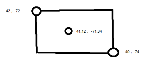
左上角坐标和右下角坐标可以绘制出一个矩形，这个矩形覆盖的范围就是要搜索的数据坐标

GET /my_index/my_type/_search
{
  "query": {
    "geo_bounding_box": {
      "location": {
        "top_left": {
          "lat": 42,
          "lon": -72
        },
        "bottom_right": {
          "lat": 40,
          "lon": -74
        }
      }
    }
  }
}

{
  "took": 117,
  "timed_out": false,
  "_shards": {
    "total": 5,
    "successful": 5,
    "failed": 0
  },
  "hits": {
    "total": 3,
    "max_score": 1,
    "hits": [
      {
        "_index": "my_index",
        "_type": "my_type",
        "_id": "2",
        "_score": 1,
        "_source": {
          "text": "Geo-point as a string",
          "location": "41.12,-71.34"
        }
      },
      {
        "_index": "my_index",
        "_type": "my_type",
        "_id": "4",
        "_score": 1,
        "_source": {
          "text": "Geo-point as an array",
          "location": [
            -71.34,
            41.12
          ]
        }
      },
      {
        "_index": "my_index",
        "_type": "my_type",
        "_id": "1",
        "_score": 1,
        "_source": {
          "text": "Geo-point as an object",
          "location": {
            "lat": 41.12,
            "lon": -71.34
          }
        }
      }
    ]
  }
}

比如 41.12,-71.34 就是一个酒店，然后我们现在搜索的是从 42,-72（代表了大厦A）和 40,-74（代表了马路 B）作为矩形的范围，在这个范围内的酒店，是什么

酒店 o2o 搜索案例以及搜索指定区域内的酒店

稍微真实点的案例，酒店 o2o app 作为一个背景，用各种各样的方式，去搜索你当前所在的地理位置附近的酒店

搜索指定区域范围内的酒店，比如说，我们可以在搜索的时候，指定两个地点，就要在东方明珠大厦和上海路组成的矩阵的范围内，搜索我想要的酒店

maping 与数据插入

PUT /hotel_app
{
    "mappings": {
        "hotels": {
            "properties": {
                "pin": {
                    "properties": {
                        "location": {
                            "type": "geo_point"
                        }
                    }
                }
            }
        }
    }
}

PUT /hotel_app/hotels/1
{
    "name": "喜来登大酒店",
    "pin" : {
        "location" : {
            "lat" : 40.12,
            "lon" : -71.34
        }
    }
}

geo_bounding_box 矩形范围搜索

上一张节讲过的

GET /hotel_app/hotels/_search
{
  "query": {
    "bool": {
      "must": [
        {
          "match_all": {}
        }
      ],
      "filter": {
        "geo_bounding_box": {
          "pin.location": {
            "top_left": {
              "lat": 40.73,
              "lon": -74.1
            },
            "bottom_right": {
              "lat": 40.01,
              "lon": -71.12
            }
          }
        }
      }
    }
  }
}

{
  "took": 2,
  "timed_out": false,
  "_shards": {
    "total": 5,
    "successful": 5,
    "failed": 0
  },
  "hits": {
    "total": 1,
    "max_score": 1,
    "hits": [
      {
        "_index": "hotel_app",
        "_type": "hotels",
        "_id": "1",
        "_score": 1,
        "_source": {
          "name": "喜来登大酒店",
          "pin": {
            "location": {
              "lat": 40.12,
              "lon": -71.34
            }
          }
        }
      }
    ]
  }
}

geo_polygon 多边形范围搜索

GET /hotel_app/hotels/_search
{
  "query": {
    "bool": {
      "must": [
        {
          "match_all": {}
        }
      ],
      "filter": {
        "geo_polygon": {
          "pin.location": {
            "points": [
              {"lat" : 40.73, "lon" : -74.1},
              {"lat" : 40.01, "lon" : -71.12},
              {"lat" : 50.56, "lon" : -90.58}
            ]
          }
        }
      }
    }
  }
}

真实地理位置坐标体验

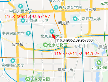
北京理工大学：116.322631,39.967157
北京交通大学：116.349652,39.957866
新街口：116.373511,39.947025

以上图片和经纬度是百度地图拾取坐标系统中获取的

PUT /hotel_app/hotels/5
{
    "name": "北京交通大学",
    "pin" : {
        "location" : {
            "lat" : 39.957866,
            "lon" : 116.349652
        }
    }
}

GET /hotel_app/hotels/_search
{
  "query": {
    "bool": {
      "must": [
        {
          "match_all": {}
        }
      ],
      "filter": {
        "geo_bounding_box": {
          "pin.location": {
            "top_left": {
              "lat": 39.967157,
              "lon": 116.322631
            },
            "bottom_right": {
              "lat": 39.947025,
              "lon": 116.373511
            }
          }
        }
      }
    }
  }
}

{
  "took": 2,
  "timed_out": false,
  "_shards": {
    "total": 5,
    "successful": 5,
    "failed": 0
  },
  "hits": {
    "total": 1,
    "max_score": 1,
    "hits": [
      {
        "_index": "hotel_app",
        "_type": "hotels",
        "_id": "5",
        "_score": 1,
        "_source": {
          "name": "北京交通大学",
          "pin": {
            "location": {
              "lat": 39.957866,
              "lon": 116.349652
            }
          }
        }
      }
    ]
  }
}

实验成功

geo_distance 实战搜索距离当前位置一定范围内的酒店

之前讲解了在某一个范围内搜索，应用场景比如：上面的图，我指定北京理工大学和新街口这两个点，要搜索这个范围内的酒店

geo_distance 是距离搜索，以一个点周围扩散的距离范围，比如我们平时使用的外卖 app、旅游的时候搜索周边旅游景点，就是这种距离当前位置搜索

搜索酒店

GET /hotel_app/hotels/_search
{
  "query": {
    "bool": {
      "must": [
        {
          "match_all": {}
        }
      ],
      "filter": {
        "geo_distance": {
          "distance": "200km",
          "pin.location": {
            "lat": 40,
            "lon": -70
          }
        }
      }
    }
  }
}

真实地理位置搜索学校

前面找了三个点，这里吧另外两个点添加进来

PUT /hotel_app/hotels/6
{
    "name": "北京理工大学",
    "pin" : {
        "location" : {
            "lat": 39.967157,
            "lon": 116.322631
        }
    }
}

PUT /hotel_app/hotels/7
{
    "name": "新街口",
    "pin" : {
        "location" : {
           "lat": 39.947025,
            "lon": 116.373511
        }
    }
}

搜索

GET /hotel_app/hotels/_search
{
  "query": {
    "bool": {
      "must": [
        {
          "match_all": {}
        }
      ],
      "filter": {
        "geo_distance": {
          "distance": "2500m",
          "pin.location": {
            "lat" : 39.957866,
            "lon" : 116.349652
          }
        }
      }
    }
  }
}


{
  "took": 2,
  "timed_out": false,
  "_shards": {
    "total": 5,
    "successful": 5,
    "failed": 0
  },
  "hits": {
    "total": 2,
    "max_score": 1,
    "hits": [
      {
        "_index": "hotel_app",
        "_type": "hotels",
        "_id": "5",
        "_score": 1,
        "_source": {
          "name": "北京交通大学",
          "pin": {
            "location": {
              "lat": 39.957866,
              "lon": 116.349652
            }
          }
        }
      },
      {
        "_index": "hotel_app",
        "_type": "hotels",
        "_id": "7",
        "_score": 1,
        "_source": {
          "name": "新街口",
          "pin": {
            "location": {
              "lat": 39.947025,
              "lon": 116.373511
            }
          }
        }
      }
    ]
  }
}

可以看到，2500 米内能找到新接口，我尝试过 3 km 的时候能把北京理工大学搜索出来

统计当前位置每个距离范围内有多少家酒店

最后一个知识点，基于地理位置进行聚合分析

比如一个需求：统计我周围几个范围内的酒店数量，如 0~100m 有几个酒店，100m~300m 有几个酒店，300m以上有几个酒店

一般来说，做酒店 app，一般来说，我们是不是会有一个地图，用户可以在地图上直接查看和搜索酒店，此时就可以显示出来举例你当前的位置，几个举例范围内，有多少家酒店，让用户知道，心里清楚，用户体验就比较好

语法如下

GET /hotel_app/hotels/_search
{
  "size": 0,
  "aggs": {
    "agg_by_distance_range": {
      "geo_distance": {
        "field": "pin.location",
        "origin": {
          "lat": 40,
          "lon": -70
        },
        "unit": "mi",
        "distance_type": "arc",
        "ranges": [
          {
            "to": 100
          },
          {
            "from": 100,
            "to": 300
          },
          {
            "from": 300
          }
        ]
      }
    }
  }
}

origin：你所在的坐标点
unit：单位

m (metres) but it can also accept: m (miles), km (kilometers)
distance_type：搜索方式，速度和精度权衡

sloppy_arc (the default), arc (most accurate) and plane (fastest)
ranges：定义范围

{
  "took": 2,
  "timed_out": false,
  "_shards": {
    "total": 5,
    "successful": 5,
    "failed": 0
  },
  "hits": {
    "total": 4,
    "max_score": 0,
    "hits": []
  },
  "aggregations": {
    "agg_by_distance_range": {
      "buckets": [
        {
          "key": "*-100.0",
          "from": 0,
          "to": 100,
          "doc_count": 1
        },
        {
          "key": "100.0-300.0",
          "from": 100,
          "to": 300,
          "doc_count": 0
        },
        {
          "key": "300.0-*",
          "from": 300,
          "doc_count": 3
        }
      ]
    }
  }
}

client 集群自动探查以及汽车零售店案例背景

快速入门篇（练习例子-员工管理），讲解过了一些基本的 java api，包括了 document 增删改查，基本的搜索，基本的聚合

高手进阶篇，必须将 java api 这块深入讲解一下，介绍一些最常用的，最核心的一些 api 的使用，用一个模拟现实的案例背景，让大家在学习的时候更加贴近业务

讲师吐槽

本段是讲师吐槽，大意是 java api 不能所有功能都讲解，只讲最常用的一些核心 api

话说在前面，我们是不可能将所有的 java api 用视频全部录制一遍的，因为 api 太多了。

我们之前讲解各种功能，各种知识点，花了那么多的时间，哪儿些才是最最关键的，知识，原理，功能，es restful api，最次最次，哪怕是搞 php，搞 python 的人也可以来学习

如果说，现在要将所有所有的 api 全部用 java api 实现一遍和讲解，太耗费时间了，几乎不可能接受

采取的粗略，将核心的 java api 语法，还有最最常用的那些 api 都给大家上课演示了

然后最后一讲，会告诉大家，在掌握了之前那些课程讲解的各种知识点之后，如果要用 java api 去实现和开发，应该怎么自己去探索和掌握

java api，api 的学习，实际上是最最简单的，纯用，没什么难度，技术难度，你掌握了课上讲解的这些 api之后，自己应该就可以举一反三，后面自己去探索和尝试出自己要用的各种功能对应的 java api 是什么。

client 集群自动探查

默认情况下，是根据我们手动指定的所有节点，依次轮询这些节点，来发送各种请求的，如下面的代码，我们可以手动为 client 指定多个节点

TransportClient client = new PreBuiltTransportClient(settings)
				.addTransportAddress(new InetSocketTransportAddress(InetAddress.getByName("localhost1"), 9300))
				.addTransportAddress(new InetSocketTransportAddress(InetAddress.getByName("localhost2"), 9300))
				.addTransportAddress(new InetSocketTransportAddress(InetAddress.getByName("localhost3"), 9300));

但是问题是，如果我们有成百上千个节点呢？难道也要这样手动添加吗？

es client 提供了一种集群节点自动探查的功能，打开这个自动探查机制以后，es client 会根据我们手动指定的几个节点连接过去，然后通过集群状态自动获取当前集群中的所有 data node，然后用这份完整的列表更新自己内部要发送请求的 node list。默认每隔 5 秒钟，就会更新一次 node list。

但是注意，es cilent 是不会将 Master node 纳入 node list 的，因为要避免给 master node 发送搜索等请求。

这样的话，我们其实直接就指定几个 master node，或者 1 个 node 就好了，client 会自动去探查集群的所有节点，而且每隔 5 秒还会自动刷新。非常棒。

:::warning 之前我记得说没有 master 之分来着，这里怎么又强调了呢？ :::

Settings settings = Settings.builder()
               .put("client.transport.sniff", true).build();
       TransportClient client = new PreBuiltTransportClient(settings)
               .addTransportAddress(new InetSocketTransportAddress(InetAddress.getByName("localhost"), 9300));

在实际的生产环境中，都是这么玩儿的。

汽车零售案例背景

简单来说，会涉及到三个数据，汽车信息、汽车销售记录、汽车 4S 店信息

后面的讲解 java api 的使用基于这个案例进行讲解

基于 upsert 实现汽车最新价格的调整

::: tip es api 的练习代码仓库地址

后面的练习代码都放在这个地址 :::

首先需要手动 mapping，既然是模拟就稍微模拟真实一点。

PUT /car_shop
{
    "mappings": {
        "cars": {
            "properties": {
                "brand": {
                    "type": "text",
                    "analyzer": "ik_max_word",
                    "fields": {
                        "raw": {
                            "type": "keyword"
                        }
                    }
                },
                "name": {
                    "type": "text",
                    "analyzer": "ik_max_word",
                    "fields": {
                        "raw": {
                            "type": "keyword"
                        }
                    }
                }
            }
        }
    }
}

brand：品牌名称，ik 中文分词，内置一个 raw 不分词字段
name：汽车名称，同上

upsert api

package cn.mrcode.newstudy.elasticsearch.senior;

import org.elasticsearch.action.ActionFuture;
import org.elasticsearch.action.index.IndexRequest;
import org.elasticsearch.action.update.UpdateRequest;
import org.elasticsearch.action.update.UpdateResponse;
import org.elasticsearch.client.transport.TransportClient;
import org.elasticsearch.common.settings.Settings;
import org.elasticsearch.common.transport.InetSocketTransportAddress;
import org.elasticsearch.common.xcontent.XContentFactory;
import org.elasticsearch.transport.client.PreBuiltTransportClient;
import org.junit.Before;
import org.junit.Test;

import java.io.IOException;
import java.net.InetAddress;
import java.net.UnknownHostException;
import java.util.concurrent.ExecutionException;


/**
 * upsert 调整汽车价格
 *
 * @author : zhuqiang
 * @date : 2019/3/13 22:19
 */
public class UpsertCarTest {
    private TransportClient client;

    @Before
    public void before() throws UnknownHostException {
        Settings settings = Settings.builder()
                .put("cluster.name", "elasticsearch") // 集群名称
                .put("client.transport.sniff", true) // 自动探查
                .build();
        client = new PreBuiltTransportClient(settings)
                .addTransportAddress(new InetSocketTransportAddress(InetAddress.getByName("localhost"), 9300));
    }

    @Test
    public void upsertCar() throws IOException, ExecutionException, InterruptedException {
        // 当 id=1 不存在的时候新增，存在的时候更新汽车价格

        IndexRequest upsertRequest = new IndexRequest("car_shop", "cars", "1");
        upsertRequest.source(
                XContentFactory.jsonBuilder()
                        .startObject()
                        .field("brand", "宝马")
                        .field("name", "宝马320")
                        .field("price", 320000)
                        .field("produce_date", "2017-01-01")
                        .endObject());

        UpdateRequest updateRequest = new UpdateRequest("car_shop", "cars", "1");
        updateRequest.doc(XContentFactory.jsonBuilder()
                .startObject()
                .field("price", 32_0000)
                .endObject())
                .upsert(upsertRequest);  // 更新的时候关联一个 upsert

        ActionFuture<UpdateResponse> update = client.update(updateRequest);
        System.out.println(update.get());

    }
}

执行更新打印的结果信息

UpdateResponse[index=car_shop,type=cars,id=1,version=1,result=created,shards=ShardInfo{total=2, successful=1, failures=[]}]

基于 mget 实现多辆汽车的配置与价格对比

场景：一般来说，我们都可以在一些汽车网站上，或者在混合销售多个品牌的汽车 4S 店的内部，都可以在系统里调出来多个汽车的信息，放在网页上，进行对比

mget：一次性将多个 document 的数据查询出来，也就是批量 id 获取

手动插入一条数据

PUT /car_shop/cars/2
{
	"brand": "奔驰",
	"name": "奔驰C200",
	"price": 350000,
	"produce_date": "2017-01-05"
}

mget 语法

@Test
public void mget() {
    MultiGetResponse responses = client.prepareMultiGet()
            .add("car_shop", "cars", "1")
            .add("car_shop", "cars", "2")
            .get();
    responses.forEach(item -> {
                GetResponse response = item.getResponse();
                if (response.isExists()) {
                    System.out.println(response.getSourceAsString());
                }
            }
    );
}

响应结果

{"brand":"宝马","name":"宝马320","price":310000,"produce_date":"2017-01-01"}
{
	"brand": "奔驰",
	"name": "奔驰C200",
	"price": 350000,
	"produce_date": "2017-01-05"
}

很奇怪的响应展示，用 java api 插入的没有格式化的 json 信息

基于 bulk 实现多 4S 店销售数据批量上传

业务场景：有一个汽车销售公司，拥有很多家 4S 店，这些 4S 店的数据，都会在一段时间内陆续传递过来，汽车的销售数据，现在希望能够在内存中缓存比如 1000 条销售数据，然后一次性批量上传到 es 中去

先手动添加两条销售数据，是重复的，模拟是重复上传的数据

PUT /car_shop/sales/1
{
    "brand": "宝马",
    "name": "宝马320",
    "price": 320000,
    "produce_date": "2017-01-01",
    "sale_price": 300000,
    "sale_date": "2017-01-21"
}

PUT /car_shop/sales/2
{
    "brand": "宝马",
    "name": "宝马320",
    "price": 320000,
    "produce_date": "2017-01-01",
    "sale_price": 300000,
    "sale_date": "2017-01-21"
}

bulk 操作

@Test
public void bulk() throws IOException {
    BulkRequestBuilder bulkRequestBuilder = client.prepareBulk();
    // 要增加一条销售数据
    bulkRequestBuilder
            .add(client.prepareIndex("car_shop", "sales", "3")
                    .setSource(XContentFactory.jsonBuilder()
                            .startObject()
                            .field("brand", "奔驰")
                            .field("name", "奔驰C200")
                            .field("price", 35_0000)
                            .field("produce_date", "2017-01-05") // 生产日期
                            .field("sale_price", 34_0000) // 销售价格
                            .field("sale_date", "2017-02-03") // 销售日期
                            .endObject()
                    )
            );
    // 修改一条数据的价格
    bulkRequestBuilder.add(client.prepareUpdate("car_shop", "sales", "1")
            .setDoc(XContentFactory.jsonBuilder()
                    .startObject()
                    .field("price", 29_0000)
                    .endObject())
    );
    // 删除一条数据，之前上传重复的数据
    bulkRequestBuilder.add(client.prepareDelete("car_shop", "sales", "2"));

    BulkResponse bulkItemResponses = bulkRequestBuilder.get();
    if (bulkItemResponses.hasFailures()) {
        System.out.println(bulkItemResponses.buildFailureMessage());
    }

    for (BulkItemResponse item : bulkItemResponses.getItems()) {
        System.out.println(item.getId() + " : " + item.getResponse().getResult());
    }
}

执行多次之后的打印结果

: UPDATED
: NOOP
: NOT_FOUND

基于 scroll 实现月度销售数据批量下载

比如说，现在要下载大批量的数据，导入到 excel 中，比如阅读、年度、销售记录等大批量数据，比如几千条、几万条、几十万条等

其实就要用到我们之前讲解的 es scroll api，对大量数据批量的获取和处理

再插入一条宝马的数据，现在就有两条宝马的数据记录了，分两次下载这两条数据

PUT /car_shop/sales/4
{
    "brand": "宝马",
    "name": "宝马320",
    "price": 320000,
    "produce_date": "2017-01-01",
    "sale_price": 280000,
    "sale_date": "2017-01-25"
}

@Test
   public void scrollTest() {
       SearchResponse searchResponse = client.prepareSearch("car_shop")
               .setTypes("sales")
               .setScroll(TimeValue.timeValueSeconds(60))
               .setQuery(QueryBuilders.termQuery("brand.keyword", "宝马"))
               .setSize(1)
               .get();

       do {
           for (SearchHit hit : searchResponse.getHits().getHits()) {
               System.out.println(hit.getSourceAsString());
           }

           searchResponse = client.prepareSearchScroll(searchResponse.getScrollId())
                   .setScroll(new TimeValue(60000))
                   .execute()
                   .actionGet();
       } while (searchResponse.getHits().getHits().length != 0);
   }

打印的数据

{
    "brand": "宝马",
    "name": "宝马320",
    "price": 320000,
    "produce_date": "2017-01-01",
    "sale_price": 280000,
    "sale_date": "2017-01-25"
}

{"brand":"宝马","name":"宝马320","price":290000,"produce_date":"2017-01-01","sale_price":300000,"sale_date":"2017-01-21"}

基于 search template 实现按品牌分页查询模板

搜索模板的功能，java api 怎么去调用一个搜索模板

elasticsearch-5.2.0\config\scripts\page-query-by-brand.mustache

{
  "from": ,
  "size": ,
  "query": {
    "match": {
      "brand.keyword": ""
    }
  }
}

::: tip 注意要重启 es，注意模板中的内容是你对应的。一定要确认不要搞错 :::

@Test
   public void pageQueryTest() {
       HashMap<String, Object> scriptParams = new HashMap<>();
       scriptParams.put("from", 0);
       scriptParams.put("size", 1);
       scriptParams.put("brand", "宝马");

       SearchTemplateResponse searchTemplateResponse = new SearchTemplateRequestBuilder(client)
               .setScriptType(ScriptType.FILE)
               .setScript("page-query-by-brand")  // page-query-by-brand.mustache
               .setScriptParams(scriptParams)
               .setRequest(new SearchRequest("car_shop").types("sales"))
               .get();
       SearchResponse response = searchTemplateResponse.getResponse();
       System.out.println(searchTemplateResponse.getResponse());
       SearchHit[] hits = response.getHits().getHits();
       for (SearchHit hit : hits) {
           System.out.println(hit.getSourceAsString());
       }
       client.close();
   }

输出信息

{"took":22,"timed_out":false,"_shards":{"total":5,"successful":5,"failed":0},"hits":{"total":2,"max_score":0.2876821,"hits":[{"_index":"car_shop","_type":"sales","_id":"4","_score":0.2876821,"_source":{
    "brand": "宝马",
    "name": "宝马320",
    "price": 320000,
    "produce_date": "2017-01-01",
    "sale_price": 280000,
    "sale_date": "2017-01-25"
}
}]}}
{
    "brand": "宝马",
    "name": "宝马320",
    "price": 320000,
    "produce_date": "2017-01-01",
    "sale_price": 280000,
    "sale_date": "2017-01-25"
}

对汽车品牌进行全文检索、精准查询和前缀搜索

为了查询，再插入一条数据

PUT /car_shop/cars/5
{
    "brand": "华晨宝马",
    "name": "宝马318",
    "price": 270000,
    "produce_date": "2017-01-20"
}

/**
 * 按品牌名搜索
 */
@Test
public void searchByBrand() {
    SearchResponse response = client.prepareSearch("car_shop")
            .setTypes("cars")
            .setQuery(QueryBuilders.matchQuery("brand", "宝马"))
            .get();
    System.out.println(response);
}

/**
 * 多字段搜索
 */
@Test
public void multiMatchQuery() {
    SearchResponse response = client.prepareSearch("car_shop")
            .setTypes("cars")
            .setQuery(QueryBuilders.multiMatchQuery("宝马", "brand", "name"))
            .get();
    System.out.println(response);
}

/**
 * terms 搜索
 */
@Test
public void commonTermsQuery() {
    SearchResponse response = client.prepareSearch("car_shop")
            .setTypes("cars")
            .setQuery(QueryBuilders.commonTermsQuery("name", "宝马320"))
            .get();
    System.out.println(response);
}

/**
 * 前缀搜索
 */
@Test
public void prefixQuery() {
    SearchResponse response = client.prepareSearch("car_shop")
            .setTypes("cars")
            .setQuery(QueryBuilders.prefixQuery("name", "宝"))
            .get();
    System.out.println(response);
}

对汽车品牌进行多种条件的组合搜索

@Test
public void boolQueryTest() {
    BoolQueryBuilder boolQueryBuilder = QueryBuilders.boolQuery()
            .must(QueryBuilders.matchQuery("brand", "宝马"))
            .mustNot(QueryBuilders.termQuery("name.keyword", "宝马318"))
            .should(QueryBuilders.termQuery("produce_date", "2017-01-02"))
            .filter(QueryBuilders.rangeQuery("price").gt(280000).lt(350000));

    SearchResponse searchResponse = client.prepareSearch("car_shop")
            .setTypes("cars")
            .setQuery(boolQueryBuilder)
            .get();
    System.out.println(searchResponse);
}

响应数据

{"took":7,"timed_out":false,"_shards":{"total":5,"successful":5,"failed":0},"hits":{"total":1,"max_score":0.18232156,"hits":[{"_index":"car_shop","_type":"cars","_id":"1","_score":0.18232156,"_source":{"brand":"宝马","name":"宝马320","price":310000,"produce_date":"2017-01-01"}}]}}

基于地理位置对周围汽车 4S 店进行搜索

要进行地理位置的搜索需要添加两个依赖

<dependency>
    <groupId>org.locationtech.spatial4j</groupId>
    <artifactId>spatial4j</artifactId>
    <version>0.6</version>                        
</dependency>

<dependency>
    <groupId>com.vividsolutions</groupId>
    <artifactId>jts</artifactId>
    <version>1.13</version>                         
    <exclusions>
        <exclusion>
            <groupId>xerces</groupId>
            <artifactId>xercesImpl</artifactId>
        </exclusion>
    </exclusions>
</dependency>

compile 'org.locationtech.spatial4j:spatial4j:0.6'
compile 'com.vividsolutions:jts:1.13'

比如我们有很多的 4s 店，给了用户一个 app，在某个地方的时候，可以根据当前的地理位置搜索一下，自己附近的 4s 店

新增一个 mapping

POST /car_shop/_mapping/shops
{
  "properties": {
      "pin": {
          "properties": {
              "location": {
                  "type": "geo_point"
              }
          }
      }
  }
}

插入数据

PUT /car_shop/shops/1
{
    "name": "上海至全宝马4S店",
    "pin" : {
        "location" : {
            "lat" : 40.12,
            "lon" : -71.34
        }
    }
}

需求：搜索两个坐标点组成的一个区域

来回顾下 restfull 语法

GET /car_shop/shops/_search
{
  "query": {
    "geo_bounding_box": {
      "pin.location": {
        "top_left": {
          "lat": 42,
          "lon": -72
        },
        "bottom_right": {
          "lat": 40,
          "lon": -74
        }
      }
    }
  }
}

再对比下 java 语法

@Test
public void geoBoundingBoxQuery() {
    GeoBoundingBoxQueryBuilder geoBoundingBoxQueryBuilder = QueryBuilders.geoBoundingBoxQuery("pin.location")
            .setCorners(40.73, -74.1, 40.01, -71.12);
    SearchResponse searchResponse = client.prepareSearch("car_shop")
            .setTypes("shops")
            .setQuery(geoBoundingBoxQueryBuilder)
            .get();
    System.out.println(searchResponse);
}

响应数据

{"took":1,"timed_out":false,"_shards":{"total":5,"successful":5,"failed":0},"hits":{"total":1,"max_score":1.0,"hits":[{"_index":"car_shop","_type":"shops","_id":"1","_score":1.0,"_source":{
    "name": "上海至全宝马4S店",
    "pin" : {
        "location" : {
            "lat" : 40.12,
            "lon" : -71.34
        }
    }
}
}]}}

需求：指定一个区域，由三个坐标点，组成，比如上海大厦，东方明珠塔，上海火车站

@Test
public void geoPolygonQuery() {
    ArrayList<GeoPoint> geoPoints = new ArrayList<>();
    geoPoints.add(new GeoPoint(40.73, -74.1));
    geoPoints.add(new GeoPoint(40.01, -71.12));
    geoPoints.add(new GeoPoint(50.56, -90.58));
    GeoPolygonQueryBuilder query = QueryBuilders.geoPolygonQuery("pin.location", geoPoints);
    SearchResponse searchResponse = client.prepareSearch("car_shop")
            .setTypes("shops")
            .setQuery(query)
            .get();
    System.out.println(searchResponse);
}

需求：搜索距离当前位置在 200 公里内的 4s 店

@Test
public void geoDistanceQuery() {
    GeoDistanceQueryBuilder query = QueryBuilders.geoDistanceQuery("pin.location")
            .point(40, -70)
            .distance(200, DistanceUnit.KILOMETERS);
    SearchResponse searchResponse = client.prepareSearch("car_shop")
            .setTypes("shops")
            .setQuery(query)
            .get();
    System.out.println(searchResponse);
}

如何自己尝试 API 以掌握所有搜索和聚合的语法

自己要什么 query，自己去用 QueryBuilders 去尝试，如 disMaxQuery
自己的某种 query，有一些特殊的参数，tieBreaker，自己拿着 query 去尝试，点一下，看 ide 的自动提示，自己扫一眼，不就知道有哪些 query，哪些参数了
如果不是 query，是聚合，也是一样的，你就拿 AggregationBuilders，点一下，看一下 ide 的自动提示，我们讲过的各种语法，都有了
包括各种聚合的参数，也是一样的，找到对应的 AggregationBuilder 之后，自己点一下，找需要的参数就可以了
自己不断尝试，就 o 了，组装了一个搜索，或者聚合，自己试一下，测一下

如果你实在找不到，搞不定，就 QQ 来找我，当然别自己一开始就跑来找我，先自己努力研究一下

有些人说，可以上官网，官网 api 也没这么全

比如大部分的语法在 QueryBuilders 中就已经支持了。所以自己根据 restfull 的写法找对应的 api

SearchResponse searchResponse = client.prepareSearch("car_shop")
               .setTypes("shops")
               .setQuery(QueryBuilders)
               .get();

快速入门篇以及高手进阶篇课程总结，以及后续阶段课程介绍

基础

快速入门：能了解最最基本的 es 的一些使用
分布式原理：了解 es 的基本原理
分布式文档系统：基本精通 es 的 document 相关的一些操作和开发
初识搜索引擎：掌握 es 最核心，最基本的一些搜索的技术
索引管理：掌握了基本的 es 的索引相关的操作
内核原理探秘：深入理解的 es 的底层的原理
Java API 初步使用：掌握最基础的 java api 的使用

开始把 es 用起来，可以玩儿起来，掌握了一些基本的知识，自己在公司做一些最最简单的小项目，也 ok

高级

深度探秘搜索技术：彻底深入的了解各种高级搜索技术，精通搜索底层原理
彻底掌握 IK 中文分词器：彻底掌握，连源码的修改都讲过了，怎么基于 mysql 热加载你的词库
深入聚合数据分析：彻底深入的掌握了各种各样的数据聚合分析的功能
数据建模实战：对模拟真实世界的有复杂关系的数据模型，讲解了建模、搜索和聚合
elasticsearch 高手进阶：高级功能，搜索模板，term vector，地理位置的搜索和聚合
java api：核心的 java api 的现场演示，如何自己去摸索所有的 java api 的使用

你做一些小型的项目，数据量不大，简单在自己公司部署几个节点的 es，3 个节点

玩儿各种各样的搜索，聚合，中文分词，有关联和层次关系的数据如何建模，document 如何管理和操作，索引的基本管理，es 的核心原理，java api 的系统的使用，高级的功能，基于地理位置的应用的开发

你都能搞定了

你只能做 es 的小型项目，或者大型项目，但是数据量大不了

后续

两个篇章

运维优化

生产环境的大规模集群的部署、运维管理、监控、安全管理、升级、性能优化、索引管理，大型 es 集群的运维知识，包括海量数据场景下的性能的调优，还有一个大数据场景的应用系统的设计，范式

搞 java 的，了解什么 es 的运维。。。。

你要是搞 java 的，结果不了解 es 运维，你也别做 es 的大型项目，大数据场景下的，你根本就不了解集群，不了解大数据集群环境下的一些特殊的配置，安全，监控，es 全景图，概览

你要是搞 java，基于 es 集群，大数据量做开发，你不了解上面这些东西，你碰到了问题，就抓瞎

你如果真是搞 java 的，最自己的技术有追求，希望自己出去找工作，技术牛逼一些，不要给自己设限制，开发，不要了解运维。如果你是个 java 架构师，你连 es 集群相关的知识都不懂，你碰到了问题，你的项目遇到了一些的报错，你都搞不定，你还当什么架构师，或者项目经理

如果你对技术有追求，就好好学一下

项目实战

各种各样的案例，作为背景，模拟现实，来用业务驱动课程的讲解，和动手的实战，更好的理解、吸收、刺激你的对技术如何运用的灵感

大型门户网站的搜索引擎系统：安全模拟真实大型搜索引擎系统的架构，特殊的点，降级，防止雪崩，缓存，架构怎么拆分，复杂的搜索引擎怎么构建，讲解

大型电商网站的数据分析系统：完全用真实的复杂的电商的业务场景，去开发一整套完整的涵盖数十个分析模块的 es 数据分析系统

后面两个篇章才是真正的拔高的地方，如果你对自己技术有追求，想把技术学好一些，建议，前面两个篇章，至少看个 2 遍，彻底掌握；后面 2 个篇章可以到时候好好看看

elasticsearch-senior

term filter 搜索数据

创建帖子数据

使用 term 搜索

查看分词

索引重建

知识总结

filter 原理剖析

1. 搜索数据，获取 document list

2. 构建 bitset

3. 遍历 bitset，查找满足条件的 documt

4. caching bitset

5. filter 大部分情况下会比 query 先执行

6. 有修改或者更新，cached bitset 自动更新

bool 组合多个 filter 搜索

第一个例子

第二个例子

总结

terms 搜索多个值

总结

range filter 范围过滤

数值范围查询

日期范围查询

总结

体验如何控制全文检索结果的精准度

1、搜索标题中包含 java 或 elasticsearch 的 blog

2、搜索标题中包含 java 和 elasticsearch 的 blog

3、搜索包含 java、elasticsearch、spark、hadoop 4 个关键字中，至少 3 个的 blog

4、用 bool 组合多个搜索条件，来搜索 title

5、bool 组合多个搜索条件，如何计算 relevance score

6、搜索 java、hadoop、spark、elasticsearch，至少包含其中 3 个关键字

总结

多关键词底层原理 term + bool

权重控制 boost

多 shard 下评分不准确大揭秘

得分不准的产生

问题产生

best fields 策略 和 dis_max

dis_max 的 tie_breaker 作用

multi_match 语法

multi_match 的 most_fiels 策略

most_fields 策略 cross-fields 搜索弊端

copy_to 解决 cross-fields

cross-fields

match_phrase 短语匹配

什么是短语匹配和近似匹配？

phrase match

term position

phrase match 基本原理

match_phrase 的 slop

语法

slop 的含义是什么？

验证 slop

混合使用 match 和近似匹配实现召回率与精准度的平衡

什么是召回率与精准度

混合使用 match 与近似匹配

rescore 机制优化近似匹配搜索的性能

match 和 phrase match（proximity match）的区别

rescore 重打分

前缀、通配符、正则搜索

前缀搜索

前缀搜索的原理

通配符搜索

正则搜索

match_phrase_prefix 实现搜索推荐

什么是搜索推荐（search-time）？

match_phrase_prefix

ngram 实现搜索推荐

什么是 ngram？

实践 ngram

TF&IDF 算法以及向量空间模型算法

boolean model

TF/IDF

vector space model

query vector

doc vector

lucene 相关度分数算法

query normalization factor

query coodination

field level boost

best fields 策略和 dis_max

`match_phrase_prefix` 实现搜索推荐

`function_score` 自定义相关度分数算法